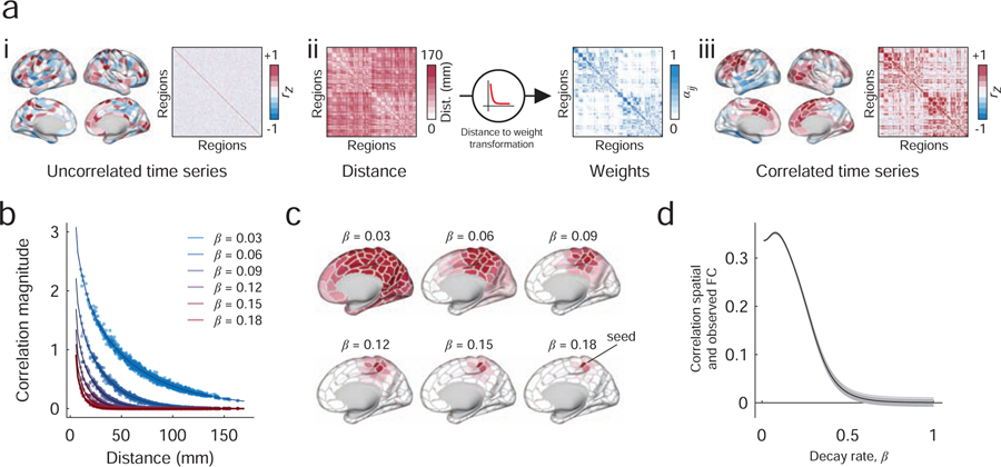
FIG. 1. Procedure for constructing matrices with distance-dependent FC.

(a) i: The procedure begins by introducing a random phase to the observed fMRI BOLD time series. This introduction is performed independently for each brain area, resulting in an uncorrelated surrogate time series. ii : Next, we generate a new surrogate time series for each brain area as the linear combination of all other time series. The weighted contribution of brain area j’s time series to that of area i depends on the distance between those two areas in three-dimensional Euclidean space, D_ij. Specifically, this distance-to-weight transformation is modeled as a decaying exponential, $w_{ij}=e^{-\beta D_{ij}}$, where β controls the decay rate. iii: This process results in spatially correlated time series. (b) The value of β controls the rate of the exponential decay and therefore parameterizes the extent to which time series exhibit more or less spatial correlation. For example, large values of β yield areal time series that are correlated with only their nearby neighbors; smaller values of β yield spatial correlations with much wider neighborhoods. (c) Examples of seed-based functional connectivity as we vary the value of β. (d) To select the value of β, we compare the similarity of the observed and spatially constrained FC patterns. The optimal value of β is the one that maximizes the correspondence between those matrices.