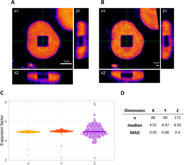
Figure 3.

Example of an isotropic cube. Orthogonal views (A) pre- and (B) post-expansion. Scale bars: 5 μm. (C) Distribution of the expansion factors calculated for each corresponding pixel line in the x-, y-, and z-dimensions for the example shown in (A) and (B). Lines represent median values. In z-dimension, we clearly see a broader distribution for the expansion factor, as the resolution in this dimension is typically lower. Single outliers that originate from the pixels at the borders of the square that were below 2 and above 10 were removed, as they are not representative of the actual expansion factor. Outliers that originated from pixel lines in the middle of the square were never removed. (D) Size, median value, and median absolute deviation (MAD) of the sample distributions plotted in (C).