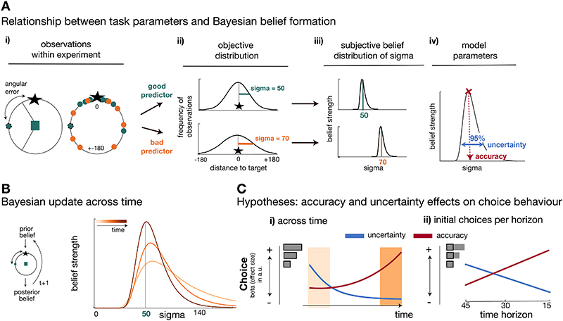
Figure 2. Task statistics, Bayesian model, and choice hypotheses.

(A) Panels depict the mapping between observations during the task (i), their statistical properties (ii), and subjective beliefs about these properties derived with Bayes’ rule (iii;iv). (A-i) A predictor’s performance can be evaluated by the angular error at each trial (left panel), and by comparing angular errors between predictors across observations (right panel). Better predictors have on average smaller angular errors (green is better than orange). (A-ii) Predictors’ angular errors were derived from normal distributions centred on the true target location. Critically, the normal distributions for good and bad predictors differed in their standard deviation (sigma): smaller sigma’s reflected smaller angular errors, i.e. more accurate predictions of the true target location. Learning about a predictor’s angular error across time corresponded to forming beliefs about a predictor’s sigma value. (A-iii) To capture this learning process, we used Bayesian modelling and derived trial-wise belief distributions over sigma for each predictor. In other words, we estimated a probability density function that expressed the belief strength in each possible sigma over a large range of sigmas, and that was updated with each new observation via Bayes’ rule. The coloured vertical lines indicate the true underlying sigmas of the predictors and the black distributions reflect the Bayesian approximation after extensive training. (A-iv) We captured two separable estimates about participants’ beliefs concerning predictors: an estimate of the accuracy of a predictor (the mode of the distribution indicated by the position of the vertical line on the abscissa) and the uncertainty in that belief (width of the belief distribution). (B) In all panels, light to dark orange represents earlier and later trials, respectively, in a block. Left: Prior beliefs are updated after observing the angular error in the trial’s outcome phase, resulting in a posterior belief. The posterior belief forms the prior for the next encounter with the same predictor. Right: Belief distribution when selecting the same predictor multiple times. Across time, the belief distribution will converge towards the true value of sigma (here, true sigma is 50). (C) Experimental hypotheses. Note that panels depict an illustration of hypothesized effect sizes of accuracy and uncertainty on choice akin to logistic GLM analyses of choice. (C-i) Participants’ patterns of explore/exploit choices should systematically change over the course of the blocks. At the beginning of a block (light orange area), participants should pursue the more uncertain predictor, that is choices should be driven by a positive uncertainty effect, but this tendency should reverse over time. Accurate predictors should be sought out throughout (positive accuracy effect), but particularly towards the end of the block (dark orange area) when the value of exploration diminishes. (C-ii) At the time of initial choices (indicated by black boxes in inset), the value of exploration should be modulated by the time horizon and choices towards uncertain predictors should systematically increase if there are more trials remaining in which to exploit the knowledge gained, i.e. in longer horizons (vice versa for accuracy-driven choices).