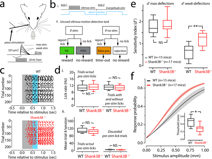
Figure 1. Vibrissa detection and stimulus hyper-reactivity in Shank3B−/−mice.
(a) Head-restrained mice were trained to lick at a waterspout when they detected vibrissa motion delivered via a piezo. The blow-up shows the shape of an individual deflection, which had a variable amplitude from trial-to-trial. (b) i) Trials in the task consisted of a variable inter-trial interval (1–6.5 seconds) after which a stimulus was presented (black trace), which coincided with the triggering of a ‘report window’ (blue). ii) Flow chart of the task. (c) Example lick of a WT (top, black dots) and Shank3B−/− (bottom, red dots) in the late stage of training. Each dot represents a lick. These lick rasters show the distribution of individual licks as dots in a given trial relative to stimulus onset. (d) i, Box-plots of mean lick rates for WT (black; n=10 mice) and Shank3B−/− (red; n=10 mice) animals. Left, shows average lick rate for trials analyzed further in the study that showed no pre-stimulus licking. Right, average lick rate but including all the trials discarded due to pre-stimulus licking. In either case, there was no significant difference in lick rates (p=0.7& p=0.8; bootstrap mean-difference test). ii, Left, Box-plots showing the average number of trials per session completed by WT (black) and Shank3B−/− (red) mice. Right, same as left, but the average number of trials that were discarded per session because of pre-stimulus licking. There was no significant difference between WT and Shank3B−/− groups for either comparison (p=0.8, left & p=0.6, right; bootstrap mean-difference test). (e) Box-plots showing the sample distributions of the detection sensitivity (d’) for strong (left) and weak (right) stimuli. Left, there was no statistical difference in the d’ for strong (1 mm) whisker deflections (WT mean ± s.e.m.: 1.79 ± 0.10; black; Shank3B−/− mean ± s.e.m.: 1.8 ±0.11, red; n=15 WT, n=17 Shank3B−/−; p=0.53; bootstrap mean-difference test). Right, Shank3B−/− mice have a significantly higher d’ for weak stimuli (WT mean ± s.e.m.: 0.59 ± 0.10; Shank3B−/− mean ± s.e.m.: 1.2 ± 0.09; n=15 WT, black; n=17 Shank3B−/− mice, red; **p<0.0001; bootstrap mean-difference test). (f) Mean psychometric curves (sigmoidal function fits) from the sessions used in e. Solid lines denote the mean, and the shaded regions are the standard error of the mean. The inset show a significant difference of detection threshold between groups (WT mean ± s.e.m.: 449 ± 42 μm; Shank3B−/− mean ± s.e.m.: 296 ± 43 μm; n=15 WT mice and 17 Shank3B−/− mice; *p=0.003; bootstrap mean-difference test; ). There was also a difference in the unitless slope-factor (WT mean ± s.e.m.: 232 ± 17 μm; Shank3B−/− mean ± s.e.m.: 149 ± 18 μm, n=15 WT mice and 17 Shank3B−/− mice; p<0.0001, bootstrap mean-difference test), which is a fit parameter related to how steep the curve is. Box-and-whisker plots show median values (middle vertical bar) and 25th (bottom side of the box) and 75th percentiles (top side of the box) with whiskers indicating the range. All bootstrap mean-difference tests were two-sided. These results repeated three times.

