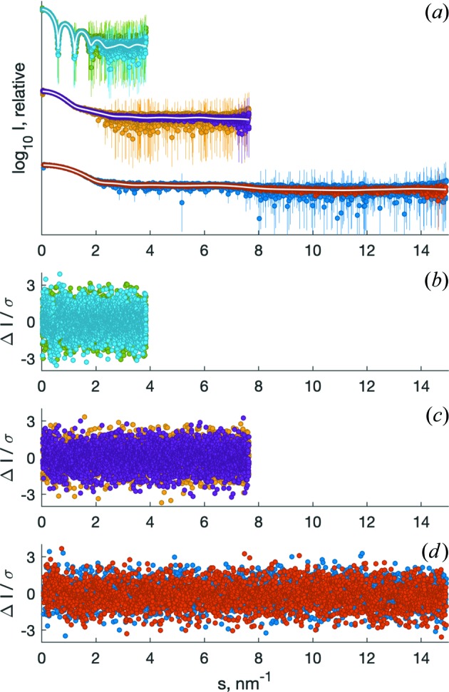
Figure 2.

Examples of simulated data from samples of varying size and shape with constant wavelength at multiple distances of the Pilatus 6M detector from the sample position. All backgrounds were generated with an exposure time of 10 s, the samples with an exposure of 1 s. (a) The simulated data of three different samples after background subtraction and scaling by concentration, offset for clarity. These are native horse spleen ferritin (1ier) at 6.0 m detector distance at a concentration of 0.5 mg ml⁻¹ (green) and 2 mg ml⁻¹ (light blue); bovine serum albumin (4f5s; Bujacz, 2012 ▸) at 3.0 m detector distance at a concentration of 0.5 mg ml⁻¹ (yellow) and 2.0 mg ml⁻¹ (violet); and myoglobin (1wla; Maurus et al., 1997 ▸) at 1.5 m detector distance at a concentration of 0.5 mg ml⁻¹ (dark blue) and 2.0 mg ml⁻¹ (red). The calculated scattering curves are overlaid in white. Error bars of all data are relative errors in logarithmic scale {SE(I)/[Ilog(10)]} and partially truncated for visibility. (b)–(d) The respective standardized residuals of the simulated data minus the calculated input scattering, divided by the error estimate. Standardized residuals are expected to be randomly distributed and to follow a standard normal distribution, i.e. >99% of all standardized residuals should be located in the range [−3; +3].