Analysis and Optimal Control of Fractional-Order Transmission of a Respiratory Epidemic Model

Abstract

The World Health Organization is yet to realise the global aim of achieving future-free and eliminating the transmission of respiratory diseases such as H1N1, SARS and Ebola since the recent reemergence of Ebola in the Democratic Republic of Congo. In this paper, a Caputo fractional-order derivative is applied to a system of non-integer order differential equation to model the transmission dynamics of respiratory diseases. The nonnegative solutions of the system are obtained by using the Generalized Mean Value Theorem. The next generation matrix approach is used to obtain the basic reproduction number ${\mathcal{R}}_0$. We discuss the stability of the disease-free equilibrium when ${\mathcal{R}}_0<1$, and the necessary conditions for the stability of the endemic equilibrium when ${\mathcal{R}}_0>1$. A sensitivity analysis shows that ${\mathcal{R}}_0$ is most sensitive to the probability of the disease transmission rate. The results from the numerical simulations of optimal control strategies disclose that the utmost way of controlling or probably eradicating the transmission of respiratory diseases should be quarantining the exposed individuals, monitoring and treating infected people for a substantial period.

Introduction

The respiratory syncytial virus, influenza virus and parainfluenza virus are some viruses that cause respiratory diseases. Influenza viruses cause more or less respiratory diseases [1]. Influenza viruses are group into Type A and Type B. The viruses are often transmitted from people and cause seasonal influenza epidemics each year. The evolving prevalence of infectious diseases is increasing every year. It occurs through the respiratory tract. The spread of the disease is rapid and widespread. Since 1980, the disease has appeared just like bird flu in Asia. The outbreak of the 2014 Ebola virus in West Africa, severe acute respiratory infectious (SARS) disease and the Middle East respiratory syndrome (MERS) caused severe impact on the health system. Most respiratory diseases have no vaccines, such as SARS and Ebola. These diseases spread quickly and may be re-infected. After the flu season, there are several different types of influenza (Types A and B) and subtypes (Type A) that circulate and cause disease. For example, the bird flu virus has several subtypes such as H5N1, H7N3, H7N7, H7N9, and H9N2, which can infect humans [1].

Epidemiological mathematical models have proven to be a valuable tool for understanding, analyzing influenza virus infection dynamics, disseminating and recommending control strategies. Although [2–6] has completed a great deal of work on dynamic modeling of influenza, it is limited to ordinary differential equations. However, currently, it has been found that the use of fractional differential equations to model many different fields of phenomena has been very successful [7–18]. For instance, in mathematical epidemiology, Ebola virus epidemic has been modeled with fractional-order differential equations by [19]. They used the SEIR fractional-order model to analyze data published by the WHO to provide projections of outbreaks in three countries in West Africa. The model considered fits precisely with the real data. Their findings revealed that the outbreak will last about two years, with an estimated 9 million infected people. Although individuals heredity play an important role in mortality rate of the disease, data analysis shows that the predicted death toll is very high.

Goufo et al. [20] took into account the stability analysis of a non-linear spread Ebola hemorrhagic fever epidemic model. They used conventional time derivatives to express models that contain new parameters that happen to be fractional. They proved that the model is well defined, poses non-negative solutions and also established the conditions for boundedness. The Routh–Hurwitz criterion was used to show the existence and stability analysis of Ebola virus model equilibrium states and showed that they strongly depend on non-linear propagation. Also, they provide the conditions for the persistence of the Ebola virus in the system. In addition, numerical simulations of non-linear propagation are provided and the results obtained are significant for combating and preventing Ebola hemorrhagic fever, which has so far caused the deaths of hundreds of families and continues to infect many people in West Africa.

Fractional diffusion mimics the human mobility network by simulating disease outbreaks [21]. Human mobility networks can smooth the spread of infectious diseases from the sidewalk to the flight route. The effort of control and removal depends on describing these networks in terms of individual connections and flux rates between the contact nodes. In some cases, transportation can be parametrized by a gravity-type model or approximated by diffuse random walks. Alternatively, they separated domestic commercial air traffic into a case study of the utility of non-diffusion heavy-tailed transport models. A new stochastic simulation of typical influenza-like infections was adopted, targeting the dense, highly connected America air travel network. They show that the mobility on the network can be defined mainly by a power law, which is consistent with the previous study. They observed that the global evolution of an outbreak on the network is precisely reproduced by a two-parameter space-fractional diffusion equation, which is determined by the air travel network. The dynamic changes of cytotoxic T-lymphocyte (CTL) responses in Ebola virus infection in vivo are described by a fractional-order model with time delay [22]. They introduced a time-delay during the CTL response period to represent the time required to simulate the immune system. Stability and Hopf bifurcation were obtained from the model through fractional Laplace transform. Moreover, the stability conditions show that the dynamics of the model can be improved by the fractional-order delay.

In [23] SIR epidemic model with non-integer order under the conditions of external noise is studied. The behavior of the system changes with the introduction of seasonality and noise force. It revealed that different non-integer order and parameters improve the dynamical behavior of the system. Multi-scale fuzzy entropy is used to study the complexity of stochastic models. They designed a hard limiter control system and simulation results which showed that with effective medical and health measures the proportion of infected people can be controlled to significantly small numbers.

Compared with integer order models, non-integer order models are more effective in modeling biological systems which have long-range and temporal memories [24]. In [25], Gonz$\acute{\text{a}}$lez-Parra et al. proposed a nonlinear order system to discuss the outbreaks of H1N1 influenza. The fractional model does not only rely on the present stage but also on all its history which makes fractional models more general than the integer-order models. They also determined that the nonlinear fractional epidemiological model can be well matched to provide numerical results that are in good agreement with the actual data for H1N1 influenza. The model suggested gives valuable facts for understanding, predicting and controlling the spread of different epidemics across the globe.

For these reasons, the fact that fractional (non-integer) order models of many phenomena have recently been shown to be more realistic than the integer order, and the fact that the fractional order also has long-range memories motivated this study. In addition, it is also obvious that modeling by fractional order derivative can capture any natural phenomena or a rich variety of dynamics observed in the system. Many of the past models focused only on the analysis of the influenza outbreaks in human populations. But, a model in which the order is an integer to describe the transmission of a respiratory epidemic has recently been proposed in [26]. However, modeling the transmission of a respiratory epidemic by fractional order model might provide a feasible alternative in controlling or probably eradicating the disease.

The present study introduces Caputo fractional-order into SEIR epidemic type of model proposed by [26]. The proposed model is analyzed without control measures to investigate its stability conditions. The sensitivity of the basic reproductive number ${\mathcal{R}}_0$ is analyzed to determine the most sensitive parameters. The interpretation of the sensitivity led us to two control measures. The optimal control theory is then used to investigate the efficiency of incorporating the control measures, namely, quarantine of exposed population and monitoring and treating of the infected population.

The remaining part of the paper is structured as follows: We provide some basic and necessary definitions about the fractional calculus in section “Fractional Calculus”. The description of the model is discussed in section “The Model”. The nonnegative solution and the stability analysis of the fractional-order differential equations are discussed in Sections “Non-negative Solutions” and “Model Equilibrium States and Stability” respectively. The optimal control of the epidemic is discussed in section “Optimal Control”. A numerical solution of the fractional model using Atanackovic and Stankovic method is discussed in section “Numerical Method”. We support our theoretical analysis with numerical simulations in section “Numerical Simulation and Discussion”. Finally, the paper concludes in section “Conclusion”.

Fractional Calculus

In this section, we define fractional integral and fractional derivative of Riemann–Liouville and Caputo respectively which are applied in this work.

Definition 1

[27]. The order $\sigma >0$ of fractional integral operator function $h:R^{+}⟶R$ defined by

$$\begin{array}{c}\hfill I^{\sigma }h(k){\displaystyle \frac{1}{\Gamma (\sigma )}}{\int }_0^k{(k-\xi )}^{\sigma -1}h(\xi )d\xi ,\end{array}$$ 1

is called the Riemann–Liouville fractional integral.

Here and elsewhere $\Gamma$ is known as the Euler gamma function and is defined as

$$\begin{array}{c}\hfill \Gamma (r)={\int }_0^{\infty }{\xi }^{r-1}{e}^{-\xi }d\xi .\end{array}$$ 2

Definition 2

[12]. The derivative function of fractional order $\sigma >0$ (where $\sigma$ lie in the half-open interval (0,1]), defined by

$$\begin{array}{c}\hfill D_{\ast a}^{\sigma }h(\xi )={\displaystyle \frac{1}{\Gamma (\lceil a\rceil -\sigma )}}{\int }_0^{\xi }{(\xi -s)}^{\lceil a\rceil -\sigma -1}\frac{d^{\lceil \sigma \rceil }}{d{s}^{\lceil \sigma \rceil }}h(s)ds.\end{array}$$ 3

is called the Caputo fractional derivative, where a is the starting point.

We use the Caputo derivative definition in this work. The initial conditions for Caputo defined fractional differential equation is the same as ordinary differential equations which is a core advantage.

The Model

Model Description

The model we studied in this work is proposed by [26]. The model considers four variables, namely, the population which is susceptible ( $S(\xi )$), the population which is exposed ($E(\xi )$), the infected population ($I(\xi )$), and the recovered population ($R(\xi )$). According to [26], $b(\xi )$ represents the rate of new susceptible people entering the population at time $\xi$, $\beta$ represents the probability of disease transmission, $\nu$ represents the seroconversion rate, $\alpha$ represents the recovery rate, ${\mu }_N$ represents the natural mortality rate, ${\mu }_D$ represents the disease induced death rate, and $\kappa$ represents the rate at which the recovered return to the susceptible population (due to the loss of immunity). These assumptions lead to the following integer-order differential equation presented by [26], where $A_r(\xi )=S(\xi )+E(\xi )+I(\xi )$ is the effective risk population at time $\xi$(or t).

$$\begin{array}{c}\hfill \left\{\begin{array}{cc}& {\displaystyle \frac{dS(\xi )}{d\xi }}=b(\xi )-\left(\beta {\displaystyle \frac{I(\xi )}{A_r(\xi )}}+{\mu }_N\right)S(\xi )+\kappa R(\xi ),\hfill \\ \hfill & {\displaystyle \frac{dE(\xi )}{d\xi }}=\beta {\displaystyle \frac{I(\xi )}{A_r(\xi )}}S(\xi )-(\nu +{\mu }_N)E(\xi ),\hfill \\ \hfill & {\displaystyle \frac{dI(\xi )}{d\xi }}=\nu E(\xi )-({\mu }_D+\alpha )I(\xi ),\hfill \\ \hfill & {\displaystyle \frac{dR(\xi )}{d\xi }}=\alpha I(\xi )-({\mu }_N+\kappa )R(\xi ).\hfill \end{array}\right.\end{array}$$ 4

The system (4) in fractional order is given by

$$\begin{array}{c}\hfill \left\{\begin{array}{cc}& D_{\ast a}^{\sigma }S(\xi )=b^{\sigma }(\xi )-\left(\beta {\displaystyle \frac{I(\xi )}{A_r(\xi )}}+{\mu }_N^{\sigma }\right)S(\xi )+{\kappa }^{\sigma }R(\xi ),\hfill \\ \hfill & D_{\ast a}^{\sigma }E(\xi )=\beta {\displaystyle \frac{I(\xi )}{A_r(\xi )}}S(\xi )-({\nu }^{\sigma }+{\mu }_N^{\sigma })E(\xi ),\hfill \\ \hfill & D_{\ast a}^{\sigma }I(\xi )={\nu }^{\sigma }E(\xi )-({\mu }_D^{\sigma }+{\alpha }^{\sigma })I(\xi ),\hfill \\ \hfill & D_{\ast a}^{\sigma }R(\xi )={\alpha }^{\sigma }I(\xi )-({\mu }_N^{\sigma }+{\kappa }^{\sigma })R(\xi ),\hfill \end{array}\right.\end{array}$$ 5

with initial conditions

$$\begin{array}{c}\hfill S(0)=S_0,E(0)=E_0,I(0)=I_0,R(0)=R_0.\end{array}$$ 6

where $D_{\ast a}^{\sigma }={\displaystyle \frac{d^{\sigma }}{d{\xi }^{\sigma }}}$ is the Caputo fractional derivative of order $\sigma$. It is important to notice that when the fractional-order $\sigma ⟶1$ , the system (5) becomes the integer-order system (4).

Non-negative Solutions

Denote ${\mathbb{R}}_{+}^4=\{Z\in {\mathbb{R}}^4:Z\ge 0\}$ and let $Z(\xi )={(S(\xi ),E(\xi ),I(\xi ),R(\xi ))}^T$. We need the following Lemma in [28] to proof non-negative solutions of system (5).

Lemma 4.1

(Generalized Mean Value Theorem [28]). Let $h(m)\in C[d,e]$ and $D_{\ast a}^{\sigma }h(m)\in C(d,e]$   for   $0<\sigma \le 1$ and $d,e\in \mathbb{R}$ then

$$\begin{array}{c}\hfill h(m)=h(d)+{\displaystyle \frac{1}{\Gamma (\sigma )}}{D}_{\ast a}^{\sigma }h(ϵ){(m-d)}^{\sigma },\end{array}$$

with $d\le ϵ\le 1,\forall m\in (d,e].$

Remark 4.1

Assume $h(m)\in C[0,e]$ and $D_{\ast a}^{\sigma }h(m)\in C(0,e]$ for $0<\sigma \le 1$. It follows from Lemma 4.1 that if $D_{\ast a}^{\sigma }h(m)\ge 0,\forall m\in (0,e)$ then h(m) is non-decreasing $\forall m\in [0,e]$, and if $D_{\ast a}^{\sigma }h(m)\le 0,\forall m\in (0,e)$ then h(m) is non-increasing $\forall m\in [0,e]$.

Theorem 1

The solution of the fractional-order initial value problem given with (5)–(6) is unique and in ${\mathbb{R}}_{+}^4$.

Proof

Using Theorem 3.1 together with Remark 3.2 in [29], we can obtain the existence and uniqueness of the solution of (5)–(6) in $(0,\infty )$. We prove that the domain ${\mathbb{R}}_{+}^4$ for the model is positively invariant, since

$$\begin{array}{cc}& D{{}^{\sigma }}_{\ast a}{S|}_{S=0}=b^{\sigma }+{\kappa }^{\sigma }R\ge 0,\hfill \\ \hfill \\ \hfill & D_{\ast a}^{\sigma }{E|}_{E=0}=\beta {\displaystyle \frac{\mathit{IS}}{S+I}}\ge 0,\hfill \\ \hfill \\ \hfill & D_{\ast a}^{\sigma }{I|}_{I=0}={\nu }^{\sigma }E\ge 0,\hfill \\ \hfill \\ \hfill & D_{\ast a}^{\sigma }{R|}_{R=0}={\alpha }^{\sigma }I\ge 0,\hfill \end{array}$$

around non-negative domain or neighborhood on each hyperplane, the vector field points to ${\mathbb{R}}_{+}^4$.$\square$

Model Equilibrium States and Stability

For the equilibrium states of the system of fractional order model (5), let

$$\begin{array}{c}\hfill \left\{\begin{array}{cc}& D_{\ast a}^{\sigma }S(\xi )=0,\hfill \\ \hfill & D_{\ast a}^{\sigma }E(\xi )=0,\hfill \\ \hfill & D_{\ast a}^{\sigma }I(\xi )=0,\hfill \\ \hfill & D_{\ast a}^{\sigma }R(\xi )=0.\hfill \end{array}\right.\end{array}$$ 7

Then the equilibrium states are $K_0=({\displaystyle \frac{b^{\sigma }}{{\mu }_N^{\sigma }}},0,0,0)$ and $K_1=(\overline{S},\overline{E},\overline{I},\overline{R})$ where

$$\begin{array}{cc}& \overline{I}={\displaystyle \frac{b^{\sigma }{\nu }^{\sigma }({\mu }_N^{\sigma }+{\kappa }^{\sigma })(({\nu }^{\sigma }+{\mu }_N^{\sigma })({\mu }_D^{\sigma }+{\alpha }^{\sigma })-\beta {\nu }^{\sigma })}{({\nu }^{\sigma }+{\mu }_N^{\sigma })({\mu }_D^{\sigma }+{\alpha }^{\sigma })(({\mu }_N^{\sigma }+{\kappa }^{\sigma })(({\nu }^{\sigma }+{\mu }_N^{\sigma })({\mu }_D^{\sigma }+{\alpha }^{\sigma })-{\mu }_N^{\sigma }({\mu }_D^{\sigma }+{\alpha }^{\sigma }+{\nu }^{\sigma })-\beta {\nu }^{\sigma })-{\kappa }^{\sigma }{\alpha }^{\sigma }{\nu }^{\sigma })+\beta {({\nu }^{\sigma })}^2{\kappa }^{\sigma }{\alpha }^{\sigma }}},\hfill \\ \hfill \\ \hfill & \overline{S}={\displaystyle \frac{b^{\sigma }{\nu }^{\sigma }({\mu }_N^{\sigma }+{\kappa }^{\sigma })-(({\mu }_N^{\sigma }+{\kappa }^{\sigma })({\nu }^{\sigma }+{\mu }_N^{\sigma })({\mu }_D^{\sigma }+{\alpha }^{\sigma })-{\kappa }^{\sigma }{\alpha }^{\sigma }{\nu }^{\sigma })\overline{I}}{{\mu }_N^{\sigma }{\nu }^{\sigma }({\mu }_N^{\sigma }+{\kappa }^{\sigma })}},\hfill \\ \hfill \\ \hfill & \overline{E}={\displaystyle \frac{({\mu }_D^{\sigma }+{\alpha }^{\sigma })\overline{I}}{{\nu }^{\sigma }}},\hfill \\ \hfill \\ \hfill & \overline{R}={\displaystyle \frac{{\alpha }^{\sigma }\overline{I}}{({\mu }_N^{\sigma }+{\kappa }^{\sigma })}}.\hfill \end{array}$$

The diseases free equilibrium state $K_0$, is where the infectives equal to zero $(I=0)$ and the endemic equilibrium state $K_1$, is where the infectives is nonzero $(I\ne 0)$.

The basic reproduction number of the system (5) using the next generation matrix approach, given by

$$\begin{array}{cc}& K=F{V}^{-1}\text{where}\hfill \\ \hfill & F=\left[{\displaystyle \frac{\partial {\mathcal{F}}_u(x_0)}{\partial x_v}}\right]\text{and}V=\left[{\displaystyle \frac{\partial {\mathcal{V}}_u(x_0)}{\partial x_v}}\right]\text{with}1\le u,v\le p,\hfill \end{array}$$

where F is non-negative and V is a non-singular M-matrix.

Applying this method on the system (5), where

$$\begin{array}{c}\hfill \mathcal{F}=\left[\begin{array}{c}{\displaystyle \frac{\beta IS}{S+E+I}}\\ 0\\ 0\\ 0\end{array}\right],\text{and}\mathcal{V}=\left[\begin{array}{c}({\nu }^{\sigma }+{\mu }_N^{\sigma })E\\ -{\nu }^{\sigma }E+({\mu }_D^{\sigma }+{\alpha }^{\sigma })I\\ -b^{\sigma }+{\displaystyle \frac{\beta IS}{S+E+I}}+{\mu }_N^{\sigma }S-{\kappa }^{\sigma }R\\ -{\alpha }^{\sigma }I+({\mu }_N^{\sigma }+{\kappa }^{\sigma })R\end{array}\right].\end{array}$$

Now, finding F and V, at disease free equilibrium, $K_0$, and using $K=F{V}^{-1}$ we have

$$\begin{array}{c}\hfill F{V}^{-1}=\left[\begin{array}{cc}{\displaystyle \frac{\beta {\nu }^{\sigma }}{({\nu }^{\sigma }+{\mu }_N^{\sigma })({\mu }_D^{\sigma }+{\alpha }^{\sigma })}}& {\displaystyle \frac{\beta }{({\mu }_D^{\sigma }+{\alpha }^{\sigma })}}\\ 0& 0\end{array}\right]\end{array}$$

Therefore, the basic reproduction number, ${\mathcal{R}}_0$, is the most dominant eigenvalue of $F{V}^{-1}$, that is,

$$\begin{array}{c}\hfill {\mathcal{R}}_0={\displaystyle \frac{\beta {\nu }^{\sigma }}{({\nu }^{\sigma }+{\mu }_N^{\sigma })({\mu }_D^{\sigma }+{\alpha }^{\sigma })}}.\end{array}$$ 8

The Jacobian matrix $J(K_0)$ for the system (5) evaluated at $K_0$ is given by

$$\begin{array}{c}\hfill J(K_0)=\left(\begin{array}{cccc}-{\mu }_N^{\sigma }& 0& -\beta & {\kappa }^{\sigma }\\ 0& -({\nu }^{\sigma }+{\mu }_N^{\sigma })& \beta & 0\\ 0& {\nu }^{\sigma }& -({\mu }_D^{\sigma }+{\alpha }^{\sigma })& 0\\ 0& 0& {\alpha }^{\sigma }& -({\mu }_N^{\sigma }+{\kappa }^{\sigma })\end{array}\right).\end{array}$$

Theorem 2

The disease free equilibrium state $K_0$ of system (5) is locally asymptotically stable if ${\displaystyle \frac{\beta {\nu }^{\sigma }}{({\nu }^{\sigma }+{\mu }_N^{\sigma })({\mu }_D^{\sigma }+{\alpha }^{\sigma })}}<1.$

Proof

The disease free equilibrium state $K_0$ is asymptotically stable locally given that the eigenvalues ${\Lambda }_l,l=1,2,3,4,$ of $J(K_0)$ satisfy the conditions [30, 31]:

$$\begin{array}{c}\hfill |arg{\Lambda }_i|>\sigma {\displaystyle \frac{\pi }{2}}.\end{array}$$ 9

We can evaluate these eigenvalues by solving the following characteristic equation

$$\begin{array}{c}\hfill \text{det}(J(K_0)-\Lambda I)=0\end{array}$$

this leads to the equation

$$\begin{array}{c}\hfill (-{\mu }_N^{\sigma }-\Lambda )({\kappa }^{\sigma }+{\mu }_N^{\sigma }+\Lambda )({\Lambda }^2+\Lambda (P+Q)+PQ-W)=0,\end{array}$$

where

$$\begin{array}{cc}\hfill P=& {\mu }_N^{\sigma }+{\nu }^{\sigma },\hfill \\ \hfill Q=& {\mu }_D^{\sigma }+{\alpha }^{\sigma },\hfill \\ \hfill W=& \beta {\nu }^{\sigma }.\hfill \end{array}$$

The characteristic equation gives the roots

$$\begin{array}{cc}\hfill {\Lambda }_1=& -{\mu }_N^{\sigma },\hfill \\ \hfill {\Lambda }_2=& -{\kappa }^{\sigma }-{\mu }_N^{\sigma },\hfill \\ \hfill {\Lambda }_{3,4}=& {\displaystyle \frac{-(P+Q)\pm \sqrt{{(P+Q)}^2-4(PQ-W)}}{2}}.\hfill \end{array}$$

Obviously, $P+Q>0$, and if $PQ>W$, then all the eigenvalues ${\Lambda }_l$, $l=1,2,3,4,$ satisfy the condition given by (9). $\square$

The basic reproduction number denoted by ${\mathcal{R}}_0$ is ${\displaystyle \frac{\beta {\nu }^{\sigma }}{({\nu }^{\sigma }+{\mu }_N^{\sigma })({\mu }_D^{\sigma }+{\alpha }^{\sigma })}}$ value and is defined as the number of cases occurring in a population which is completely susceptible. Biologically, if ${\mathcal{R}}_0$ is less than one, then the infection will disappear, but if it is more than one, the infection still exists.

For the discussion of the asymptotic stability of the persistence of the disease of system (5), we need the following definition and Lemma 5.1.

Definition 3

[32].The discriminant D(h) of a polynomial

$$\begin{array}{c}\hfill h(y)=y^m+c_1{y}^{m-1}+c_2{y}^{m-2}+\cdots +c_m\end{array}$$ 10

is defined by $D(h)={(-1)}^{m(m-1)/2}R(h,h^{\prime })$, where $h^{\prime }$ is the derivative of h. If $f(y)=y^{\xi }+d_1{y}^{\xi -1}+d_2{y}^{\xi -2}+\cdots +d_m$,R(h, f) is the determinant of the corresponding Sylvester $(m+\xi )\otimes (m+\xi )$ matrix, the Sylvester matrix is formed by filling the matrix beginning with the upper left corner with the coefficients of h(y) and then shifting down one row and one column to the right side. The process is then repeated for the coefficients of f(y) .

Lemma 5.1

[32]. For the polynomial equation,

$$\begin{array}{c}\hfill H(\Lambda )={\Lambda }^m+b_1{\Lambda }^{m-1}+b_2{\Lambda }^{m-2}+\cdots +b_m=0,\end{array}$$ 11

the conditions displayed below make all the roots of (11) satisfy (9):

1. for $m=1$, the condition for (11) is $b_1>0$

2. for $m=2$, the conditions for (11) are either Routh–Hurwitz conditions or $b_1<0$ $4b_2>{(b_1)}^2$, $|{tan}^{-1}\left({\displaystyle \frac{\sqrt{4b_2-{(b_1)}^2}}{b_1}}\right)|>{\displaystyle \frac{\sigma \pi }{2}}$;

3. for $m=3$, if the discriminant of $H(\Lambda ),D(H)$ is positive, then Routh–Hurwitz conditions are the necessary and sufficient conditions for (11), i.e.

   $b_1>0,b_3>0,b_1{b}_2>b_{3}ifD(H)>0.$

4. If $D(H)<0$,  $b_1\ge 0$,  $b_3>0$, $\sigma <2/3$ , then the condition (11) is satisfied. Also if $D(H)<0$, $b_1<0$, $b_2<0$, $\sigma >2/3$, then all roots of $P(\lambda )=0$ satisfies $|arg(\Lambda )|<\sigma \pi /2$.

5. If $D(H)<0$, $b_1>0$, $b_2>0$, $b_1{b}_2=b_3$ then condition (11) is satisfied for all $\sigma \in [0,1)$.

6. For general m, $b_m>0$ is a necessary condition for condition (11) to be satisfied.

The Jacobian matrix $J(K_1)$ calculated at the disease persistence equilibrium is given as:

$$\begin{array}{c}\hfill J(K_1)=\left(\begin{array}{cccc}{\displaystyle \frac{\beta \overline{I}\overline{S}}{{(\overline{S}+\overline{E}+\overline{I})}^2}}-{\displaystyle \frac{\beta \overline{I}}{\overline{S}+\overline{E}+\overline{I}}}-{\mu }_N^{\sigma }& {\displaystyle \frac{\beta \overline{I}\overline{S}}{{(\overline{S}+\overline{E}+\overline{I})}^2}}& -({\displaystyle \frac{\beta }{\overline{S}+\overline{E}+\overline{I}}}-{\displaystyle \frac{\beta \overline{I}}{{(\overline{S}+\overline{E}+\overline{I})}^2}})\overline{S}& {\kappa }^{\sigma }\\ -{\displaystyle \frac{\beta \overline{I}\overline{S}}{{(\overline{S}+\overline{E}+\overline{I})}^2}}+{\displaystyle \frac{\beta \overline{I}}{\overline{S}+\overline{E}+\overline{I}}}& -({\displaystyle \frac{\beta \overline{I}\overline{S}}{{(\overline{S}+\overline{E}+\overline{I})}^2}}+{\nu }^{\sigma }+{\mu }_N^{\sigma })& {\displaystyle \frac{\beta \overline{S}}{\overline{S}+\overline{E}+\overline{I}}}-{\displaystyle \frac{\beta \overline{I}\overline{S}}{{(\overline{S}+\overline{E}+\overline{I})}^2}}& 0\\ 0& {\nu }^{\sigma }& -({\mu }_D^{\sigma }+{\alpha }^{\sigma })& 0\\ 0& 0& {\alpha }^{\sigma }& -({\mu }_N^{\sigma }+{\kappa }^{\sigma })\end{array}\right).\end{array}$$

By using the characteristic equation $\text{det}(J(K_1)-\Lambda I)=0$, the linearized system above is in the form

$$\begin{array}{c}\hfill H(\Lambda )={\Lambda }^4+d_1{\Lambda }^3+d_2{\Lambda }^2+d_3\Lambda +d_4=0,\end{array}$$ 12

where

$$\begin{array}{cc}\hfill d_1=& {\displaystyle \frac{1}{\overline{S}+\overline{E}+\overline{I}}}((3\overline{E}+3\overline{S}+3\overline{I}){\mu }_N^{\sigma }+({\nu }^{\sigma }+\beta +{\alpha }^{\sigma }+{\kappa }^{\sigma }+{\mu }_D^{\sigma })\overline{I}\hfill \\ \hfill & +({\nu }^{\sigma }+{\alpha }^{\sigma }+{\kappa }^{\sigma }+{\mu }_D^{\sigma })(\overline{E}+\overline{S})),\hfill \\ \hfill d_2=& {\displaystyle \frac{1}{\overline{S}+\overline{E}+\overline{I}}}((3\overline{E}+3\overline{S}+3\overline{I}){({\mu }_N^{\sigma })}^2+((2{\nu }^{\sigma }+2\beta +3{\alpha }^{\sigma }+2{\kappa }^{\sigma }+3{\mu }_D^{\sigma })\overline{I}\hfill \\ \hfill & +2(\overline{E}+\overline{S})({\nu }^{\sigma }+{\displaystyle \frac{3}{2}}{\alpha }^{\sigma }\hfill \\ \hfill & +{\kappa }^{\sigma }+{\displaystyle \frac{3}{2}}{\mu }_D^{\sigma })){\mu }_N^{\sigma }+((\beta +{\alpha }^{\sigma }+{\kappa }^{\sigma }+{\mu }_D^{\sigma }){\nu }^{\sigma }+(\beta +{\alpha }^{\sigma }+{\mu }_D^{\sigma }){\kappa }^{\sigma }\hfill \\ \hfill & +\beta ({\alpha }^{\sigma }+{\mu }_D^{\sigma }))\overline{I}+(({\alpha }^{\sigma }+{\kappa }^{\sigma }+{\mu }_D^{\sigma }){\nu }^{\sigma }\hfill \\ \hfill & +{\kappa }^{\sigma }({\alpha }^{\sigma }+{\mu }_D^{\sigma }))\overline{E}-\overline{S}((\beta -{\alpha }^{\sigma }-{\kappa }^{\sigma }-{\mu }_D^{\sigma }){\nu }^{\sigma }-{\kappa }^{\sigma }({\alpha }^{\sigma }+{\mu }_D^{\sigma }))),\hfill \\ \hfill d_3=& {\displaystyle \frac{1}{{(\overline{S}+\overline{E}+\overline{I})}^2}}({(\overline{S}+\overline{E}+\overline{I})}^2{({\mu }_N^{\sigma })}^3+(\overline{S}+\overline{E}+\overline{I})(({\nu }^{\sigma }\hfill \\ \hfill & +\beta +3{\alpha }^{\sigma }+{\kappa }^{\sigma }+3{\mu }_D^{\sigma })\overline{I}\hfill \\ \hfill & +({\nu }^{\sigma }+3{\alpha }^{\sigma }+{\kappa }^{\sigma }+3{\mu }_D^{\sigma })(\overline{E}+\overline{S})){({\mu }_N^{\sigma })}^2\hfill \\ \hfill & +(((\beta +2{\alpha }^{\sigma }+{\kappa }^{\sigma }+2{\mu }_D^{\sigma }){\nu }^{\sigma }+(\beta +2{\alpha }^{\sigma }+2{\mu }_D^{\sigma }){\kappa }^{\sigma }\hfill \\ \hfill & +2\beta ({\alpha }^{\sigma }+{\mu }_D^{\sigma }))\overline{I^2}+((\beta +4{\alpha }^{\sigma }+2{\kappa }^{\sigma }+4{\mu }_D^{\sigma }){\nu }^{\sigma }\hfill \\ \hfill & +(\beta +4{\alpha }^{\sigma }+4{\mu }_D^{\sigma }){\kappa }^{\sigma }+2\beta ({\alpha }^{\sigma }+{\mu }_D^{\sigma }))\overline{E}\hfill \\ \hfill & +4\overline{S}(({\alpha }^{\sigma }+{\displaystyle \frac{1}{2}}{\kappa }^{\sigma }+{\mu }_D^{\sigma }){\nu }^{\sigma }+({\displaystyle \frac{1}{4}}\beta +{\alpha }^{\sigma }+{\mu }_D^{\sigma }){\kappa }^{\sigma }\hfill \\ \hfill & +{\displaystyle \frac{1}{2}}\beta ({\alpha }^{\sigma }+{\mu }_D^{\sigma }))\overline{I}+2((({\alpha }^{\sigma }+{\displaystyle \frac{1}{2}}{\kappa }^{\sigma }+{\mu }_D^{\sigma }){\nu }^{\sigma }\hfill \\ \hfill & +{\kappa }^{\sigma }({\alpha }^{\sigma }+{\mu }_D^{\sigma }))\overline{E}-\overline{S}((\beta -{\alpha }^{\sigma }-{\displaystyle \frac{1}{2}}{\kappa }^{\sigma }-{\mu }_D^{\sigma }){\nu }^{\sigma }-{\kappa }^{\sigma }({\alpha }^{\sigma }+{\mu }_D^{\sigma })))(\overline{E}+\overline{S})){\mu }_N^{\sigma }\hfill \\ \hfill & +(((\beta +{\alpha }^{\sigma }+{\mu }_D^{\sigma }){\kappa }^{\sigma }+\beta ({\alpha }^{\sigma }+{\mu }_D^{\sigma })){\nu }^{\sigma }+{\kappa }^{\sigma }\beta ({\alpha }^{\sigma }+{\mu }_D^{\sigma }))\overline{I^2}+(((\beta +2{\alpha }^{\sigma }+2{\mu }_D^{\sigma }){\kappa }^{\sigma }\hfill \\ \hfill & +\beta ({\alpha }^{\sigma }+{\mu }_D^{\sigma })){\nu }^{\sigma }+{\kappa }^{\sigma }\beta ({\alpha }^{\sigma }+{\mu }_D^{\sigma }))\overline{E}+2\overline{S}{\kappa }^{\sigma }({\alpha }^{\sigma }+{\mu }_D^{\sigma })({\nu }^{\sigma }+{\displaystyle \frac{1}{2}}\beta ))\overline{I}\hfill \\ \hfill & +{\kappa }^{\sigma }(\overline{E}+\overline{S})(({\alpha }^{\sigma }+{\mu }_D^{\sigma })\overline{E}-\overline{S}(\beta -{\alpha }^{\sigma }-{\mu }_D^{\sigma })){\nu }^{\sigma }),\hfill \\ \hfill d_4=& {\displaystyle \frac{1}{{(\overline{S}+\overline{E}+\overline{I})}^2}}({(\overline{S}+\overline{E}+\overline{I})}^2({\alpha }^{\sigma }+{\mu }_D^{\sigma }){({\mu }_N^{\sigma })}^3+(({\alpha }^{\sigma }+{\mu }_D^{\sigma })({\nu }^{\sigma }+\beta +{\kappa }^{\sigma }){\overline{I}}^2\hfill \\ \hfill & +2({\alpha }^{\sigma }+{\mu }_D^{\sigma })(\overline{E}+\overline{S})({\nu }^{\sigma }+{\displaystyle \frac{1}{2}}\beta +{\kappa }^{\sigma })\overline{I}+(({\alpha }^{\sigma }+{\mu }_D^{\sigma })({\nu }^{\sigma }+{\kappa }^{\sigma })\overline{E}\hfill \\ \hfill & -\overline{S}((\beta -{\alpha }^{\sigma }-{\mu }_D^{\sigma }){\nu }^{\sigma }-{\kappa }^{\sigma }({\alpha }^{\sigma }+{\mu }_D^{\sigma })))(\overline{E}+\overline{S})){({\mu }_N^{\sigma })}^2\hfill \\ \hfill & +(((\beta +{\kappa }^{\sigma }){\nu }^{\sigma }+{\kappa }^{\sigma }\beta )({\alpha }^{\sigma }+{\mu }_D^{\sigma }){\overline{I}}^2+({\alpha }^{\sigma }+{\mu }_D^{\sigma })(((\beta +2{\kappa }^{\sigma }){\nu }^{\sigma }\hfill \\ \hfill & +{\kappa }^{\sigma }\beta )\overline{E}+2\overline{S}{\kappa }^{\sigma }({\nu }^{\sigma }+{\displaystyle \frac{1}{2}}\beta ))\overline{I}+(\overline{E}+\overline{S}){\kappa }^{\sigma }(({\alpha }^{\sigma }+{\mu }_D^{\sigma })\overline{E}-\overline{S}(\beta -{\alpha }^{\sigma }-{\mu }_D^{\sigma })){\nu }^{\sigma }){\mu }_N^{\sigma }\hfill \\ \hfill & +{\nu }^{\sigma }\overline{I}\beta {\kappa }^{\sigma }{\mu }_D^{\sigma }(\overline{E}+\overline{I})).\hfill \end{array}$$

Let D(H) be the discriminant of the polynomial H, then based on the definition 3, we obtain the discriminant of H as

$$\begin{array}{cc}\hfill D(H)=& \left|\begin{array}{ccccccc}1& d_1& d_2& d_3& d_4& 0& 0\\ 0& 1& d_1& d_2& d_3& d_4& 0\\ 0& 0& 1& d_1& d_2& d_3& d_4\\ 4& 3d_1& 2d_2& d_3& 0& 0& 0\\ 0& 4& 3d_1& 2d_2& d_3& 0& 0\\ 0& 0& 4& 3d_1& 2d_2& d_3& 0\\ 0& 0& 0& 4& 3d_1& 2d_2& d_3\\ \end{array}\right|\hfill \\ \hfill & =256{d_4}^3+{d_4}^2(-27{d_1}^4+144{d_1}^2{d}_2-192d_1{d}_3-128{d_2}^2)\hfill \\ \hfill & +d_4(18{d_1}^3{d}_2{d}_3+{d_1}^2(-4{d_2}^3-6{d_3}^2-80d_1{d_2}^2{d}_3+16{d_2}^4+144d_2{d_3}^2)\hfill \\ \hfill & -4{d_1}^3{d_3}^3+{d_1}^2{d_2}^2{d_3}^2+18d_1{d}_2{d_3}^3-4{d_2}^3{d_3}^2-27{d_3}^4.\hfill \end{array}$$

Lemma 5.2

From condition (6) in Lemma 5.1 the positive equilibrium point $K_1$ is locally asymptotically stable, since the polynomial $H(\Lambda )$ as given in (12) has a coefficients $d_1$, $d_2$, $d_3$, and $d_4$ positives.

A Sensitivity Analysis of ${\mathcal{R}}_0$

Here, we investigate the response of ${\mathcal{R}}_0$ to parameter changes and determine the effect of each parameter on ${\mathcal{R}}_0$ and the potential for effective control and elimination of the disease. It is straightforward to calculate the partial derivatives of the value of ${\mathcal{R}}_0$ using Eq. (8) with respect to the parameters $\beta ,{\nu }^{\sigma },b^{\sigma },{\mu }_N^{\sigma },{\mu }_D^{\sigma }$ and the recovery rate ${\alpha }^{\sigma }$. With all other parameters held constant, the elasticity $E_x$ (or the variable’s normalized forward sensitivity index) approximates the fractional change in ${\mathcal{R}}_0$ that results from a unit fractional change in parameter x, defined as

$$\begin{array}{c}\hfill E_x={\displaystyle \frac{x}{{\mathcal{R}}_0}}·{\displaystyle \frac{\partial {\mathcal{R}}_0}{\partial x}}.\end{array}$$

This index shows how sensitive ${\mathcal{R}}_0$ is to changes of parameter x. Specifically, a positive (negative) index shows that an increase in the parameter value results in an increase (decrease) of ${\mathcal{R}}_0$ [33].

The elasticities for the quantities of interest are

$$\begin{array}{cc}\hfill E_{\beta }& =1\hfill \end{array}$$ 13

$$\begin{array}{cc}\hfill E_{{\nu }^{\sigma }}& =1-{\displaystyle \frac{{\nu }^{\sigma }}{({\nu }^{\sigma }+{\mu }_N^{\sigma })}}\hfill \end{array}$$ 14

$$\begin{array}{cc}\hfill E_{{\mu }_N^{\sigma }}& =-{\displaystyle \frac{{\mu }_N^{\sigma }}{({\nu }^{\sigma }+{\mu }_N^{\sigma })}}\hfill \end{array}$$ 15

$$\begin{array}{cc}\hfill E_{{\mu }_D^{\sigma }}& =-{\displaystyle \frac{{\mu }_D^{\sigma }}{({\mu }_D^{\sigma }+{\alpha }^{\sigma })}}\hfill \end{array}$$ 16

$$\begin{array}{cc}\hfill E_{{\alpha }^{\sigma }}& =-{\displaystyle \frac{{\alpha }^{\sigma }}{{\mu }_D^{\sigma }+{\alpha }^{\sigma }}}\hfill \end{array}$$ 17

Figure 1 indicate that, ${\mathcal{R}}_0$ is most sensitive to $\beta$ the disease transmission rate, followed by ${\alpha }^{\sigma }$ the recovery rate. The seroconversion rate ${\nu }^{\sigma }$ and the natural death rate ${\mu }_N^{\sigma }$ have the same sensitivity index. It can also be observed that, ${\mathcal{R}}_0$ is least sensitive to ${\mu }_D^{\sigma }$, the disease induced death rate.

Fig. 1.

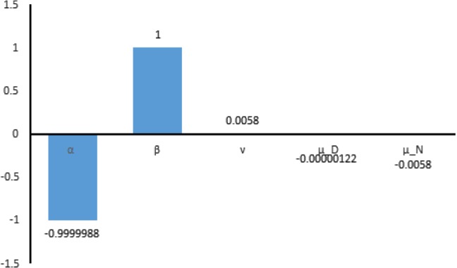
The sensitivity analysis of the basic reproductive number

In detail, the sensitivity indexes for ${\alpha }^{\sigma }$, $\beta$, ${\nu }^{\sigma }$, ${\mu }_D^{\sigma }$, and ${\mu }_N^{\sigma }$, are found to be $-0.9999988$, 1, 0.0058, $-0.00000122$, and $-0.0058$ respectively, once all parameters are fixed at their baseline values (Fig. 1). Thus, for instance, if the rate of recovery were to increase or (decrease) by $10\%$, then the value of ${\mathcal{R}}_0$ would decrease or (increase) by $9.999988\%$. Likewise, a $10\%$ increase or (decrease) of the disease transmission rate would correspond to a $10\%$ decrease or (increase) of the ${\mathcal{R}}_0$, $10\%$ increase or (decrease) of seroconversion rate would decrease or (increase) the ${\mathcal{R}}_0$ by $0.058\%$, $10\%$ increase or (decrease) of the disease induced death rate would correspond to decrease or (increase) the value of ${\mathcal{R}}_0$ by $0.0000122\%$ and $10\%$ increase or (decrease) of the natural death rate would correspond to a $0.058\%$ decrease or (increase) in the value of ${\mathcal{R}}_0$.

Therefore, the above interpretations recommend that control strategies that can efficiently decrease the probability of disease transmission $\beta$, natural death rate ${\mu }_N^{\sigma }$, disease induced death rate ${\mu }_D^{\sigma }$, should be used to control the disease transmission effectively. Additionally, increase the rate of recovery ${\alpha }^{\sigma }$ will lead to a decrease in ${\mathcal{R}}_0$, thus all control strategies that can effectively help reduce the transmission of the respiratory diseases should be applied. The mathematical perspective for these strategies would be detailed in our subsequent model.

Optimal Control

In this section, we extend our model in Eq. (6) by introducing two time-dependent control measures, namely $u_1(\xi )$ (quarantine of exposed population groups) and $u_2(\xi )$ (monitoring and treatment of infected populations ). It is assumed that the exposed population is reduced by the factor $(1-u_1(\xi ))$ as they are quarantine. Furthermore, the infected population is reduced by a factor of $(1-u_2(\xi ))$ as they are monitored and treated by health professionals. The model system (6) becomes

$$\begin{array}{cc}\hfill D_{\ast a}^{\sigma }S=& b^{\sigma }-(\beta {\displaystyle \frac{I}{S+E+I}}(1-u_1)+{\mu }_N^{\sigma })S+{\kappa }^{\sigma }R,\hfill \\ \hfill D_{\ast a}^{\sigma }E=& \beta {\displaystyle \frac{I}{S+E+I}}(1-u_1)S-({\nu }^{\sigma }(1-u_2)+{\mu }_N^{\sigma })E,\hfill \\ \hfill D_{\ast a}^{\sigma }I=& {\nu }^{\sigma }(1-u_2)E-({\mu }_D^{\sigma }+{\alpha }^{\sigma })I,\hfill \\ \hfill D_{\ast a}^{\sigma }R=& {\alpha }^{\sigma }I-({\mu }_N^{\sigma }+{\kappa }^{\sigma })R,\hfill \end{array}$$

with the given objective function

$$\begin{array}{c}\hfill J(u_1,u_2)={\int }_0^T(c_{1}E+c_{2}I+c_3{u}_1^2+c_4{u}_2^2)d\xi ,\end{array}$$ 18

where E is the exposed population and I is the infected population. T is the final time and the coefficients $c_1,c_2,c_3,c_4$ are positive weights. Our aim is to minimize the exposed and infected population while minimizing the cost of control $u_1,u_2$. Thus, we search for an optimal control $u_1^{\ast },u_2^{\ast }$, such that

$$\begin{array}{c}\hfill J(u_1^{\ast },u_2^{\ast })=\underset{u_1,u_2}{min}\{J(u_1,u_2)|u_1,u_2\in \Omega \}\end{array}$$ 19

where the control set is

$$\begin{array}{c}\hfill \Omega =\{(u_1,u_2)|u_i:[0,T]⟶[0,\infty )\text{Lebesgue measurable,}i=1,2,\}.\end{array}$$

The terms $c_{1}E$ and $c_{2}I$ represent the cost of reducing the exposed and infected population respectively, while $c_3{u}_1^2$ is the cost of quarantine and also, $c_4{u}_2^2$ is the cost of monitoring and treatment. The necessary conditions that an optimal control must satisfy come from the Pontryagin’s Minimum Principle [34–37]. This principle converts Eqs. (6) and (18) into a problem of point-wise minimizing a Hamiltonian M with respect to $(u_1,u_2)$ stated as follows:

$$\begin{array}{cc}\hfill M=& c_{1}E+c_{2}I+c_3{u}_1^2+c_4{u}_2^2\hfill \\ \hfill & +{\lambda }_S\{b^{\sigma }-(\beta {\displaystyle \frac{I}{S+E+I}}(1-u_1)+{\mu }_N^{\sigma })S+{\kappa }^{\sigma }R\}\hfill \\ \hfill & +{\lambda }_E\{\beta {\displaystyle \frac{I}{S+E+I}}(1-u_1)S-({\nu }^{\sigma }(1-u_2)+{\mu }_N^{\sigma })E\}\hfill \\ \hfill & +{\lambda }_I\{{\nu }^{\sigma }(1-u_2)E-({\mu }_D^{\sigma }+{\alpha }^{\sigma })I\}\hfill \\ \hfill & +{\lambda }_R\{{\alpha }^{\sigma }I-({\mu }_N^{\sigma }+{\kappa }^{\sigma })R\},\hfill \end{array}$$

where ${\lambda }_S$, ${\lambda }_E$, ${\lambda }_I$ and ${\lambda }_R$, adjoint variables or co-state variables [34–37]

$$\begin{array}{cc}& -{\displaystyle \frac{d{\lambda }_S}{d\xi }}={\displaystyle \frac{\partial M}{\partial S}}={\lambda }_S\left(\frac{\beta I\left(1-u_1\right)S}{{\left(S+E+I\right)}^2}-\frac{\beta I(\xi )\left(1-u_1\right)}{S+E+I}-{\mu }_N^{\sigma }\right)\hfill \\ \hfill & +{\lambda }_E\left(-\frac{\beta I\left(1-u_1\right)S}{{\left(S+E+I\right)}^2}+\frac{\beta I\left(1-u_1\right)}{S+E+I}\right)\hfill \\ \hfill & -{\displaystyle \frac{d{\lambda }_E}{d\xi }}={\displaystyle \frac{\partial M}{\partial E}}=c_1+\frac{{\lambda }_S\beta I\left(1-u_1\right)S}{{\left(S+E+I\right)}^2}\hfill \\ \hfill & +{\lambda }_E\left(-\frac{\beta I\left(1-u_1\right)S}{{\left(S+E+I\right)}^2}-{\nu }^{\sigma }\left(1-u_2\right)-{\mu }_N^{\sigma }\right)+{\lambda }_I{\nu }^{\sigma }\left(1-u_2\right)\hfill \\ \hfill & -{\displaystyle \frac{d{\lambda }_I}{d\xi }}={\displaystyle \frac{\partial M}{\partial I}}=c_2-{\Lambda }_S\left(\frac{\beta \left(1-u_1\right)}{S+E+I}-\frac{\beta I\left(1-u_1\right)}{{\left(S+E+I\right)}^2}\right)S\hfill \\ \hfill & +{\lambda }_E\left(\frac{\beta \left(1-u_1\right)S}{S+E+I}-\frac{\beta I\left(1-u_1\right)S}{{\left(S+E+I\right)}^2}\right)\hfill \\ \hfill & +{\lambda }_I\left(-{\mu }_D^{\sigma }-{\alpha }^{\sigma }\right)+{\lambda }_R{\alpha }^{\sigma }\hfill \\ \hfill & -{\displaystyle \frac{d{\lambda }_R}{d\xi }}={\displaystyle \frac{\partial M}{\partial R}}={\lambda }_S{\kappa }^{\sigma }+{\lambda }_R\left(-{\mu }_N^{\sigma }-{\kappa }^{\sigma }\right)\hfill \end{array}$$

The transversality conditions are ${\lambda }_S(T)={\lambda }_E(T)={\lambda }_I(T)={\lambda }_R=0.$

On the interior of the control set, where $0<u_i<1$, for $i=1,2$ we have

$$\begin{array}{cc}& {\displaystyle \frac{\partial M}{\partial u_1}}=2c_3{u}_1+{\displaystyle \frac{{\lambda }_S\beta IS}{S+E+I}}-{\displaystyle \frac{{\lambda }_E\beta IS}{S+E+I}}=0,\hfill \\ \hfill & {\displaystyle \frac{\partial M}{\partial u_2}}=E{\nu }^{\sigma }{\lambda }_E-E{\nu }^{\sigma }{\lambda }_I+2c_4{u}_2=0.\hfill \end{array}$$

We obtain

$$\begin{array}{cc}\hfill u_1=& {\displaystyle \frac{1}{2}}{\displaystyle \frac{SI\beta \left({\lambda }_E-{\lambda }_S\right)}{\left(S+E+I\right)c_3}},\hfill \\ \hfill u_2=& {\displaystyle \frac{1}{2}}{\displaystyle \frac{-E{\nu }^{\sigma }{\lambda }_E+E{\nu }^{\sigma }{\lambda }_I}{c_4}}.\hfill \\ \hfill \end{array}$$

Theorem 3

The control parameters $(u_1^{\ast },u_2^{\ast })$ that minimizes $J(u_1,u_2)$ over $\mathcal{U}$ is given by

$$\begin{array}{cc}& u_1^{\ast }=max\{0,min(1,{\displaystyle \frac{1}{2}}{\displaystyle \frac{SI\beta \left({\lambda }_E-{\lambda }_S\right)}{\left(S+E+I\right)c_3}})\},\hfill \\ \hfill & u_2^{\ast }=max\{0,min(1,{\displaystyle \frac{1}{2}}{\displaystyle \frac{-E{\nu }^{\sigma }{\lambda }_E+E{\nu }^{\sigma }{\lambda }_I}{c_4}})\},\hfill \\ \hfill \end{array}$$

where ${\lambda }_S,{\lambda }_E,{\lambda }_I$ and ${\lambda }_R$ are the adjoint variables satisfying (6) and the following transversality conditions: ${\lambda }_S(T)={\lambda }_E(T)={\lambda }_I(T)={\lambda }_R(T)=0$ and

$$\begin{array}{c}\hfill u_1^{\ast }=\{\begin{array}{ccc}0\hfill & \text{if}\hfill & u_1\le 0\hfill \\ u_1,\hfill & \text{if}\hfill & 0<u_1<1\hfill \\ 1,\hfill & \text{if}\hfill & u_1,\ge 1\hfill \end{array}{u}_2^{\ast }=\{\begin{array}{ccc}0\hfill & \text{if}\hfill & u_2\le 0\hfill \\ u_2,\hfill & \text{if}\hfill & 0<u_2<1\hfill \\ 1,\hfill & \text{if}\hfill & u_2,\ge 1.\hfill \end{array}\end{array}$$

Numerical Method

Atanackovic and Stankovic [38] numerical method FDE is discussed in this section. This method indicates that the fractional derivative of a function $f(\xi )$ with order $\sigma$ may be stated as

$$\begin{array}{cc}\hfill D_{\ast a}^{\sigma }g(\xi )=& {\displaystyle \frac{1}{\Gamma (2-\sigma )}}\times \{{\displaystyle \frac{g^{(1)}(\xi )}{{\xi }^{\sigma -1}}}[1+\sum _{k=1}^{\infty }{\displaystyle \frac{\Gamma (k-1+\sigma )}{\Gamma (\sigma -1)k!}}]-[{\displaystyle \frac{\sigma -1}{{\xi }^{\sigma }}}g(\xi )\hfill \\ \hfill & +\sum _{k=2}^{\infty }{\displaystyle \frac{\Gamma (k-1+\sigma )}{\Gamma (\sigma -1)(k-1)!}}\times ({\displaystyle \frac{g(\xi )}{{\xi }^{\sigma }}}+{\displaystyle \frac{V_k(g)(\xi )}{{\xi }^{k-1+\sigma }}})]\},\hfill \end{array}$$ 20

where

$$\begin{array}{c}\hfill V_k(g)(\xi )=-(k-1){\int }_0^{\xi }{\tau }^{k-2}g(\tau )d\tau ,k=2,3,\cdots ,\end{array}$$ 21

with the following properties:

$$\begin{array}{c}\hfill {\displaystyle \frac{d}{d\xi }}{V}_k(g)=-(k-1){\xi }^{k-2}g(\xi ),k=2,3,\cdots ,\end{array}$$ 22

By using K terms with the sums appearing in (20), we can approximate $D^{\sigma }g(\xi )$ as

$$\begin{array}{cc}\hfill D_{\ast a}^{\sigma }g(\xi )=& {\displaystyle \frac{1}{\Gamma (2-\sigma )}}\times \{{\displaystyle \frac{g^{(1)}(\xi )}{g^{\sigma -1}}}[1+\sum _{k=1}^K{\displaystyle \frac{\Gamma (k-1+\sigma )}{\Gamma (\sigma -1)k!}}]-[{\displaystyle \frac{\sigma -1}{{\xi }^{\sigma }}}g(\xi )\hfill \\ \hfill & +\sum _{k=2}^K{\displaystyle \frac{\Gamma (k-1+\sigma )}{\Gamma (\sigma -1)(k-1)!}}\times ({\displaystyle \frac{g(\xi )}{{\xi }^{\sigma }}}+{\displaystyle \frac{V_k(g)(\xi )}{{\xi }^{k-1+\sigma }}})]\}.\hfill \end{array}$$

The above equation can be written as

$$\begin{array}{c}\hfill D_{\ast a}^{\sigma }g(\xi )\simeq \Omega (\sigma ,\xi ,K)g^{(1)}(\xi )+\Theta (\sigma ,\xi ,K)g(\xi )+\sum _{k=2}^{K}B(\sigma ,\xi ,K){\displaystyle \frac{V_k(g)(\xi )}{{\xi }^{k-1+\sigma }}},\end{array}$$ 23

where

$$\begin{array}{cc}\hfill \Omega (\sigma ,\xi ,K)& ={\displaystyle \frac{1+{\sum }_{k=1}^K\frac{\Gamma (k-1+\sigma )}{\Gamma (\sigma -1)k!}}{\Gamma (2-\sigma ){\xi }^{\sigma -1}}},\hfill \\ \hfill Z(\sigma ,\xi )& ={\displaystyle \frac{1}{{\xi }^{\sigma }\Gamma (2-\sigma )}},\hfill \\ \hfill B(\sigma ,\xi ,k)& =-{\displaystyle \frac{\Gamma (k-1+\sigma )}{\Gamma (2-\sigma )\Gamma (\sigma -1)(k-1)!}},\hfill \\ \hfill \Theta (\sigma ,\xi ,K)& =Z(a,\xi )+\sum _{k=2}^K{\displaystyle \frac{B(\sigma ,\xi ,k)}{{\xi }^{\sigma }}}.\hfill \end{array}$$

We set

$$\begin{array}{cc}& {\Theta }_1(\xi )=S(\xi ),{\Theta }_k(\xi )=V_k(S)(\xi ),\hfill \\ \hfill & {\Theta }_{K+1}(\xi )=E(\xi ),{\Theta }_{K+k}(\xi )=V_k(E)(\xi ),\hfill \\ \hfill & {\Theta }_{2K+1}(\xi )=I(\xi ),{\Theta }_{2K+k}(\xi )=V_k(I)(\xi ),\hfill \\ \hfill & {\Theta }_{3K+1}(\xi )=R(\xi ),{\Theta }_{3K+k}(\xi )=V_k(R)(\xi ),\hfill \end{array}$$ 24

for $k=2,3,\cdots$ We can rewrite system (7) as

$$\begin{array}{c}\hfill \begin{array}{cc}& \Omega (\sigma ,\xi ,K){\Theta }_1^{{}^{\prime }}(\xi )+\Phi (\sigma ,\xi ,K){\Theta }_1(\xi )+\sum _{k=2}^{K}B(\sigma ,\xi ,k){\displaystyle \frac{{\Theta }_k(\xi )}{{\xi }^{k-1+\sigma }}}\hfill \\ \hfill & =b^{\sigma }(\xi )-\left({\displaystyle \frac{\beta {\Theta }_{2K+1}(\xi )}{{\Theta }_1(\xi )+{\Theta }_{K+1}(\xi )+{\Theta }_{2K+1}(\xi )}}+{\mu }_N^{\sigma }\right){\Theta }_1(\xi )+{\kappa }^{\sigma }{\Theta }_{3K+1}(\xi ),\hfill \\ \hfill & \omega (\sigma ,\xi ,K){\Theta }_{K+1}^{{}^{\prime }}(\xi )+\Phi (\sigma ,\xi ,K){\Theta }_{K+1}(\xi )\hfill \\ \hfill & +\sum _{k=2}^{K}B(\sigma ,\xi ,K){\displaystyle \frac{{\Theta }_{K+m}(\xi )}{{\xi }^{k-1+\sigma }}}\hfill \\ \hfill & ={\displaystyle \frac{\beta {\Theta }_{2K+1}(\xi )}{{\Theta }_1(\xi )+{\Theta }_{K+1}(\xi )+{\Theta }_{2K+1}(\xi )}}{\Theta }_1(\xi )-({\nu }^{\sigma }+{\mu }_N^{\sigma }){\Theta }_{K+1}(\xi ),\hfill \\ \hfill & \omega (\sigma ,\xi ,K){\Theta }_{2K+1}^{{}^{\prime }}(\xi )+\Phi (\sigma ,\xi ,K){\Theta }_{2K+1}(\xi )\hfill \\ \hfill & +\sum _{k=2}^{K}B(\sigma ,\xi ,K){\displaystyle \frac{{\Theta }_{2K+k}(\xi )}{{\xi }^{k-1+\sigma }}}\hfill \\ \hfill & ={\nu }^{\sigma }{\Theta }_{K+1}(\xi )-({\mu }_D^{\sigma }+{\alpha }^{\sigma }){\Theta }_{2k+1}(\xi ),\hfill \\ \hfill & \omega (\sigma ,\xi ,K){\Theta }_{3K+1}^{{}^{\prime }}(\xi )+\Phi (\sigma ,\xi ,K){\Theta }_{3K+1}(\xi )+\sum _{k=2}^{K}B(\sigma ,\xi ,K){\displaystyle \frac{{\Theta }_{3K+k}(\xi )}{{\xi }^{k-1+\sigma }}}\hfill \\ \hfill & ={\alpha }^{\sigma }{\Theta }_{2K+1}(\xi )-({\mu }_N^{\sigma }+{\kappa }^{\sigma }){\Theta }_{3K+1}(\xi ),\hfill \end{array}\end{array}$$ 25

where

$$\begin{array}{c}\hfill \begin{array}{cc}\hfill {\Theta }_k(\xi )& =-(k-1){\int }_0^{\xi }{\psi }^{k-2}S(\psi )d\psi ,\hfill \\ \hfill {\Theta }_{K+k}(\xi )& =-(k-1){\int }_0^{\xi }{\psi }^{k-2}E(\psi )d\psi ,\hfill \\ \hfill {\Theta }_{2K+k}(\xi )& =-(k-1){\int }_0^{\xi }{\psi }^{k-2}I(\psi )d\psi ,\hfill \\ \hfill {\Theta }_{3K+k}(\xi )& =-(k-1){\int }_0^{\xi }{\psi }^{k-2}R(\psi )d\psi ,\hfill \\ \hfill k& =2,3,\cdots ,K.\hfill \end{array}\end{array}$$ 26

Now we can rewrite (23) and (25) as follows:

$$\begin{array}{c}\hfill \begin{array}{cc}\hfill {\Theta }_1^{\prime }(\xi )& ={\displaystyle \frac{1}{\Omega (\sigma ,\xi ,K)}}[b^{\sigma }(\xi )\hfill \\ \hfill & -\left({\displaystyle \frac{\beta {\Theta }_{2K+1}(\xi )}{{\Theta }_1(\xi )+{\Theta }_{K+1}(\xi )+{\Theta }_{2K+1}(\xi )}}+{\mu }_N^{\sigma }+\Phi (\sigma ,\xi ,K)\right){\Theta }_1(\xi )\hfill \\ \hfill & +{\kappa }^{\sigma }{\Theta }_{3K+1}(\xi )-\sum _{k=2}^{K}B(\sigma ,\xi ,K){\displaystyle \frac{{\Theta }_m(\xi )}{{\xi }^{k-1+\sigma }}}],\hfill \\ \hfill {\Theta }_k^{\prime }(\xi )& =-(k-1){\xi }^{k-2}{\Theta }_1(\xi ),k=2,3,\cdots ,K,\hfill \\ \hfill {\Theta }_{K+1}^{\prime }(\xi )& ={\displaystyle \frac{1}{\Omega (\sigma ,\xi ,K)}}[{\displaystyle \frac{\beta {\Theta }_{2K+1}(\xi )}{{\Theta }_1(\xi )+{\Theta }_{K+1}(\xi )+{\Theta }_{2K+1}(\xi )}}{\Theta }_1(\xi )\hfill \\ \hfill & -({\nu }^{\sigma }+{\mu }_N^{\sigma }+\Phi (\sigma ,\xi ,K)){\Theta }_{K+1}\hfill \\ \hfill & -\sum _{k=2}^{K}B(\sigma ,\xi ,K){\displaystyle \frac{{\Theta }_{K+m}(\xi )}{{\xi }^{k-1+\sigma }}}],\hfill \\ \hfill {\Theta }_{K+k}^{\prime }(\xi )& =-(k-1){\xi }^{k-2}{\Theta }_{K+1}(\xi ),k=2,3,\cdots ,K,\hfill \\ \hfill {\Theta }_{2K+1}^{\prime }(\xi )& ={\displaystyle \frac{1}{\Omega (\sigma ,\xi ,K)}}[{\nu }^{\sigma }{\Theta }_{K+1}(\xi )-({\mu }_D^{\sigma }+{\alpha }^{\sigma }+\Phi (\sigma ,\xi ,K)){\Theta }_{2K+1}(\xi )\hfill \\ \hfill & -\sum _{k=2}^{K}B(\sigma ,\xi ,K){\displaystyle \frac{{\Theta }_{2K+k}(\xi )}{{\xi }^{k-1+\sigma }}}],\hfill \\ \hfill & {\Theta }_{2K+k}^{\prime }(\xi )=-(k-1){\xi }^{k-2}{\Theta }_{2K+1}(\xi ),k=2,3,\cdots ,K,\hfill \\ \hfill {\Theta }_{3K+1}^{\prime }(\xi )& ={\displaystyle \frac{1}{\Omega (\sigma ,\xi ,K)}}[{\alpha }^{\sigma }{\Theta }_{2K+1}(\xi )-({\mu }_N^{\sigma }+{\kappa }^{\sigma }+\Phi (\sigma ,\xi ,K)){\Theta }_{3K+1}(\xi )\hfill \\ \hfill & -\sum _{k=2}^{K}B(\sigma ,\xi ,K){\displaystyle \frac{{\Theta }_{3K+k}(\xi )}{{\xi }^{k-1+\sigma }}}],\hfill \\ \hfill {\Theta }_{3K+k}^{\prime }(\xi )& =-(k-1){\xi }^{k-2}{\Theta }_{3K+1}(\xi ),k=2,3,\cdots ,K,\hfill \end{array}\end{array}$$ 27

with the initial conditions

$$\begin{array}{c}\hfill \begin{array}{cc}\hfill {\Theta }_1(\delta )& =S_0,{\Theta }_k(\delta )=0,k=2,3,\cdots ,K,\hfill \\ \hfill {\Theta }_{K+1}(\delta )& =E_0,{\Theta }_{K+k}(\delta )=0,k=2,3,\cdots ,M,\hfill \\ \hfill {\Theta }_{2K+1}(\delta )& =I_0,{\Theta }_{2K+k}(\delta )=0,k=2,3,\cdots ,K,\hfill \\ \hfill {\Theta }_{3K+1}(\delta )& =R_0,{\Theta }_{3K+k}(\delta )=0,k=2,3,\cdots ,K.\hfill \end{array}\end{array}$$ 28

The system (27) with (28) can be solved numerically by using the Runge-Kutta fourth order method.

Numerical Simulation and Discussion

In this section, we present numerical simulations to confirm the theoretical results obtained in the preceding section.

By using the well known generalized Euler method (GEM) [39] with values in Table 1, we simulate system (5).

Table 1.

Parameter values

Parameter	Discription	Value
$b^{\sigma }(\xi )$	Recruitment rate into the susceptible population at time $\xi$	0.061/day [26]
$\beta$	Probability of disease transmission	1.1/day [40]
${\nu }^{\sigma }$	Rate of seroconversion (from expose to infectious)	0.004107/day [26]
${\alpha }^{\sigma }$	Rate of recovery	0.7222/day [26]
${\kappa }^{\sigma }$	Rate of loss of immunity	0.95 [26]
${\mu }_N^{\sigma }$	Natural death rate	0.000024/day [26]
${\mu }_D^{\sigma }$	Disease induced death rate	0.00000088/day [26]

For the parameter values in Table 1 above and by calculation, we obtained ${\mathcal{R}}_0=1.5143$ and the endemic equilibrium $K_1=(1679.128,858.647,4.883,3.712)$.

We obtained ${\mathcal{R}}_0=1.5143$, $D(P)=2.389>0$ and the simulations in Fig. 2 show that the endemic equilibrium $K_1$ is positive and locally asymptotically stable for $\sigma =0.70$, $\sigma =0.80$, $\sigma =0.90$ and $\sigma =1.0$, satisfying condition 6 of Lemma 5.1. It can obviously be seen in Fig. 2 that, compared with the situation of order $\sigma =0.70$ and $\sigma =0.80$, the trajectory of the system with order $\sigma =0.90$ is nearer to the trajectory of the system with the order $\sigma =1.0$. Thus, the bigger of the trajectory difference, the distant from $\sigma$ to 1.0.

Fig. 2.

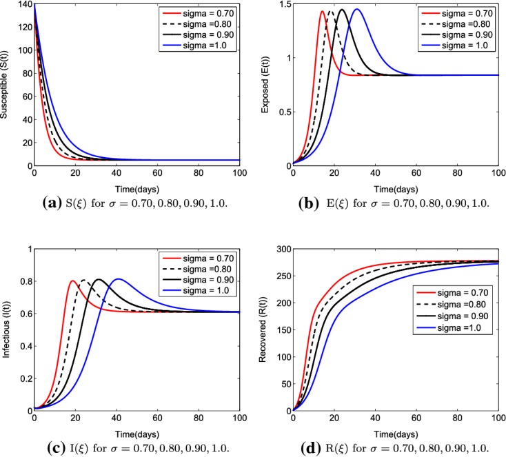
The figures show the trajectories for the state variables ($S(\xi ),E(\xi ),I(\xi ),R(\xi )$) of system (5) for different order values

It can be seen from Fig. 3 when $\sigma =1$ system (5) is the classical integer-order system (4). The display of the trajectories indicates the behavior of the approximate solutions for system (5) obtained for the value of $\sigma =1$.

Fig. 3.

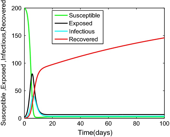
The approximate solution of $S(\xi ),E(\xi ),I(\xi ),R(\xi )$, against time for $\sigma =1$

The Effects of Optimal Control Strategies on the Exposed and Infected Populations

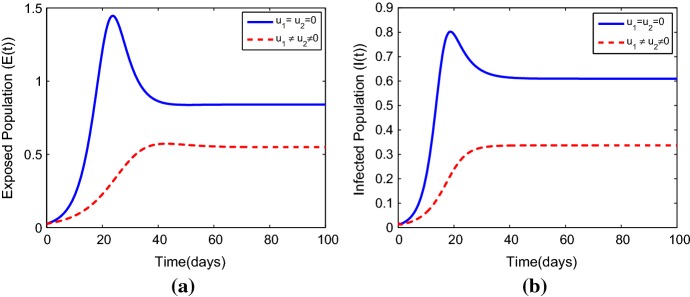
It can be seen from Fig. 4 that the optimal control $u_1$ and $u_2$ has a significant effect on the exposed and the infected populations respectively. Infection level is reduced rapidly but not eliminated. This suggests that monitoring and treatment strategies that can allow the immune response to rebuilding should also be well-thought-out (Figs. 5, 6).

Fig. 4.

The simulations displaying the result of $u_1$ (quarantine of the exposed population groups) and $u_2$ (monitoring and treatment of the infected people) on a exposed populations, b infected populations

Fig. 5.

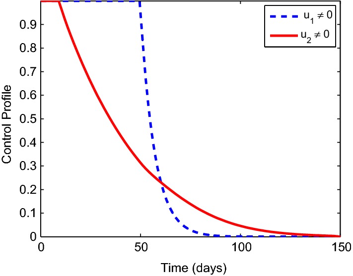
Simulation displaying the optimal control profile $u_1$ and $u_2$. The $u_1$ indicates control profile of quarantine of the exposed population’s whiles $u_2$ indicates control profile of monitoring and treating the infected populations

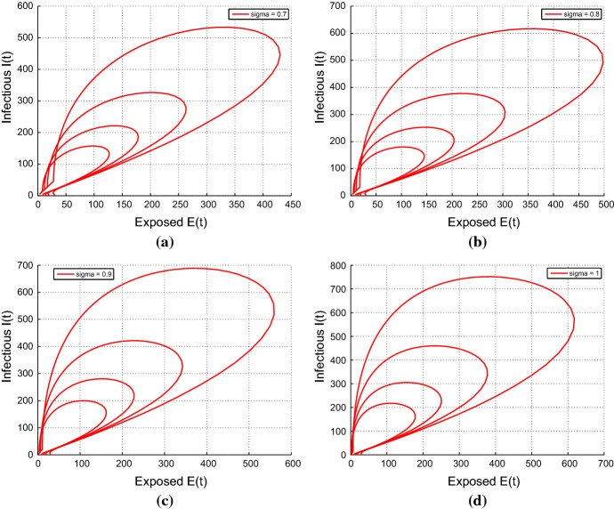
Fig. 6.

This shows the phase portrait for fractional-order model with $\sigma =0.70,0.80,0.90,1.0$

Conclusion

We introduced Caputo fractional-order into a classical integer-order model proposed by [26] to model the transmission dynamics of respiratory disease. The nonnegative solution of the model is provided by using the generalized mean value theorem. We obtained the basic reproductive number ${\mathcal{R}}_0$, which perform as a threshold parameter in the disease control. We established and investigated the stability analysis of the fractional-order model with respect to the values of ${\mathcal{R}}_0$. The disease-free equilibrium is locally asymptotically stable if ${\mathcal{R}}_0<1$. For ${\mathcal{R}}_0>1$, using Lemma 5.1 and condition 6, we investigated the local stability of the positive endemic equilibrium state. Sensitivity analysis shows that ${\mathcal{R}}_0$ is most sensitive to the disease transmission rate $\beta$. This recommends that periodic monitoring by medical professionals and researchers should be done to control the transmission of the disease. Additionally, we investigated the optimal control problem by the application of the optimal control theory. We used the Pontryagin’s Minimum Principle to provide the necessary conditions needed for the existence of the optimal solution to the optimal control problem. Also, we applied the Atanackovic and Stankovic method to provide a numerical solution to system (5). Lastly, the theoretical results were verified by numerical simulations to measure the efficacy and impact of control on the transmission of the respiratory diseases. From the numerical simulation, the size of the infected population is significantly reduced under the controlled conditions. This proposes that if all two control measures $u_1$ (quarantine of exposed population groups) and $u_2$ (monitoring and treatment of infected populations) are employed for the same period of time and continue for a considerable period of time, the future of free from transmission of a respiratory disease could be achieved. In this manner, the fractional-order optimal control method can progress the value of the treatment (Fig. 7).

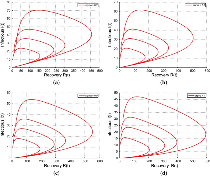
Fig. 7.

This shows the phase portrait for fractional-order model with $\sigma =0.70,0.80,0.90,1.0$

The major advantages of our proposed fractional order model which cannot be exhibited by classical order model are:

• It’s highly effective and efficient which help us to obtain better results.

• It’s easy to implement.

• It provides improved precision of the process model by offering more flexibility in model identification.

• By modeling system by fractional order we can model a higher system by low order model.

• It has the effect of memory, which is essential factor in many biological processes.

References

- 1.Pongsumpum P. Simple model for respiratory diseases. Int. J. Biosci. Biochem. Bioinform. 2017;7:118–128. [Google Scholar]
- 2.Tan X, Yuan L, Zhou J, Zheng Y, Yang F. Modeling the initial transmission dynamics of influenza A H1N1 in Guangdong Province, China. Int. J. Infect. Dis. 2013;17:479–484. doi: 10.1016/j.ijid.2012.11.018. [DOI] [PubMed] [Google Scholar]
- 3.Lee J, Chowell G, Jung E. A dynamic compartmental model for the Middle East respiratory syndrome outbreak in the Republic of Korea: a retrospective analysis on control interventions and superspreading events. J. Theor. Biol. 2016;408:118–126. doi: 10.1016/j.jtbi.2016.08.009. [DOI] [PMC free article] [PubMed] [Google Scholar]
- 4.Gaffey RH, Viboud C. Application of the CDC EbolaResponse modeling tool to disease predictions. Epidemics. 2018;22:22–28. doi: 10.1016/j.epidem.2017.03.001. [DOI] [PMC free article] [PubMed] [Google Scholar]
- 5.Samsuzzoha M, Singh M, Lucy D. Parameter estimation of Influenza epidemic model. Appl. Math. Comput. 2013;220:616–629. [Google Scholar]
- 6.Liu S, Pang L, Ruan S, Zhang X. Global dynamics of avian influenza epidemic models with psychological effect. Comput. Math. Methods Med. 2015;2015:1–12. doi: 10.1155/2015/913726. [DOI] [PMC free article] [PubMed] [Google Scholar]
- 7.Jajarmi A, Baleanu D. A new fractional analysis on the interaction of HIV with CD4+ T-cells. Chaos Solitons Fractals. 2018;113:221–229. doi: 10.1016/j.chaos.2018.06.009. [DOI] [Google Scholar]
- 8.Baleanu D, Jajarmi A, Bonyah E, Hajipour M. New aspects of the poor nutrition in the life cycle within the fractional calculus. Adv. Differ. Eqs. 2018;2018:1–14. doi: 10.1186/s13662-017-1452-3. [DOI] [Google Scholar]
- 9.Baleanu D, Asad JH, Jajarmi A. New aspects of the motion of a particle in a circular cavity. Proc. Rom. Acad. Ser. A. 2018;19:361–367. [Google Scholar]
- 10.Jajarmi A, Baleanu D. Suboptimal control of fractional-order dynamic systems with delay argument. J. Vib. Control. 2018;24:2430–2446. doi: 10.1177/1077546316687936. [DOI] [Google Scholar]
- 11.Baleanu D, Jajarmi A, Hajipour M. On the nonlinear dynamical systems within the generalized fractional derivatives with Mittag–Leffler kernel. Nonlinear Dyn. 2018;94:397–414. doi: 10.1007/s11071-018-4367-y. [DOI] [Google Scholar]
- 12.Diethelm K. A fractional calculus based model for the simulation of an outbreak of dengue fever. Nonlinear Dyn. 2013;71:613–61. doi: 10.1007/s11071-012-0475-2. [DOI] [Google Scholar]
- 13.Yusuf A, Qureshi S, Inc M, Aliyu AI, Baleanu D, Shaikh AA. Two-strain epidemic model involving fractional derivative with Mittag–Leffler kernel. Chaos: Interdiscip. J. Nonlinear Sci. 2018;28:123121. doi: 10.1063/1.5074084. [DOI] [PubMed] [Google Scholar]
- 14.Abro KA, Memon AA, Memon AA. Functionality of circuit via modern fractional differentiations. Analog Integr. Circuits Signal Process. 2019;99:11–21. doi: 10.1007/s10470-018-1371-6. [DOI] [Google Scholar]
- 15.Aliyu AI, Inc M, Yusuf A, Baleanu D. A fractional model of vertical transmission and cure of vector-borne diseases pertaining to the Atangana–Baleanu fractional derivatives. Chaos Solitons Fractals. 2018;116:268–277. doi: 10.1016/j.chaos.2018.09.043. [DOI] [Google Scholar]
- 16.Arafa AAM, Rida SZ, Khalil M. The effect of anti-viral drug treatment of human immunodeficiency virus type 1 (HIV-1) described by a fractional order model. Appl. Math. Model. 2013;37:2189–2196. doi: 10.1016/j.apm.2012.05.002. [DOI] [Google Scholar]
- 17.Özalp N, Demirci E. A fractional order SEIR model with vertical transmission. Math. Comput. Model. 2011;54:1–6. doi: 10.1016/j.mcm.2010.12.051. [DOI] [Google Scholar]
- 18.Goufo EFD, Maritz R, Munganga J. Some properties of the Kermack–McKendrick epidemic model with fractional derivative and nonlinear incidence. Adv. Differ. Equ. 2014;278:1–9. [Google Scholar]
- 19.Area, I., Batarfi, H., Losada, J., Nieto, J.J., Shammakh, W., Torres, Á.: On a fractional-order Ebola epidemic model. Adv. Differ. Equ. 1–12 (2015)
- 20.Goufo EFD, Pane MK, Mugisha S. Stability analysis of epidemic models of Ebola hemorrhagic fever with non-linear transmission. J. Nonlinear Sci. Appl. 2016;9:4191–4205. doi: 10.22436/jnsa.009.06.61. [DOI] [Google Scholar]
- 21.Gustafson, K.B., Bayati, B.S., Eckhoff, P.A.: Fractional diffusion emulates a human mobility network during a simulated disease outbreak. Institute for Disease Modeling, Intellectual Ventures, Bellevue, WA, USA (2016)
- 22.Latha VP, Rihan FA, Rakkiyappan R, Velmurugan G. A fractional-order delay differential model for Ebola infection and CD T-cells response: stability analysis and Hopf bifurcation. Int. J. Biomath. 2017;10:22p. doi: 10.1142/S179352451750111X. [DOI] [Google Scholar]
- 23.He S, Banerjee S. Epidemic outbreaks and its control using a fractional order model with seasonality and stochastic infection. Physica A. 2018;501:408–417. doi: 10.1016/j.physa.2018.02.045. [DOI] [Google Scholar]
- 24.Latha VP, Rihan FA, Rakkiyappan R, Velmurugan G. A fractional-order model for Ebola virus infection with delayed immune response on heterogeneous complex networks. J. Comput. Appl. Math. 2018;339:134–146. doi: 10.1016/j.cam.2017.11.032. [DOI] [Google Scholar]
- 25.González-Parra G, Arenas AJ, Chen-Charpentier BM. A fractional-order epidemic model for the simulation of outbreaks of influenza A(H1N1) Math. Methods Appl. Sci. 2014;37:2218–2226. doi: 10.1002/mma.2968. [DOI] [Google Scholar]
- 26.Costa PJ. Applied Mathematics for the Analysis of Biomedical Data: Models, Methods, and MATLAB. London: Wiley; 2017. [Google Scholar]
- 27.Petras I. Fractional-Order Nonlinear Systems: Modeling, Analysis and Simulation. New York: Springer; 2011. [Google Scholar]
- 28.Odibat ZM, Shawagfeh NT. Generalized Taylor’s formula. Appl. Math. Comput. 2007;186:286–293. [Google Scholar]
- 29.Lin W. Global existence theory and chaos control of fractional differential equations. J. Math. Anal. Appl. 2007;332:709–726. doi: 10.1016/j.jmaa.2006.10.040. [DOI] [Google Scholar]
- 30.Ahmed E, El-Sayed AMA, El-Saka HAA. Equilibrium points, stability and numerical solutions of fractional-order predator-prey and rabies models. J. Math. Anal. Appl. 2007;325:542–553. doi: 10.1016/j.jmaa.2006.01.087. [DOI] [Google Scholar]
- 31.Matignon, D.: Stability results for fractional differential equations with applications to control processing. In: Computational Engineering in Systems Applications Lille, France. 2, p. 963 (1996)
- 32.Ahmed E, Elgazzar AS. On fractional-order differential equations model for nonlocal epidemics. Physica A. 2007;379:607–614. doi: 10.1016/j.physa.2007.01.010. [DOI] [PMC free article] [PubMed] [Google Scholar]
- 33.Chitnis N, Hyman JM, Cushing JM. Determining important parameters in the spread of malaria through the sensitivity analysis of a mathematical model. Bull. Math. Biol. 2008;70:1272–1296. doi: 10.1007/s11538-008-9299-0. [DOI] [PubMed] [Google Scholar]
- 34.Sajjadi SS, Pariz N, Karimpour A, Jajarmi A. An off-line NMPC strategy for continuous-time nonlinear systems using an extended modal series method. Nonlinear Dyn. 2014;78:2651–2674. doi: 10.1007/s11071-014-1616-6. [DOI] [Google Scholar]
- 35.Jajarmi A, Nayyeri MD, Nik HS. A novel feedforward-feedback suboptimal control of linear time-delay systems. J. Complex. 2016;35:46–62. doi: 10.1016/j.jco.2016.02.001. [DOI] [Google Scholar]
- 36.Jajarmi A, Hajipour M. An efficient finite difference method for the time-delay optimal control problems with time-varying delay. Asian J. Control. 2017;19:554–563. doi: 10.1002/asjc.1371. [DOI] [Google Scholar]
- 37.Pontryagin LS, Boltyanskii VG, Gamkrelidze RV, Mishchenko EF. The Mathematical Theory of Optimal Processes. New York: Wiley; 1962. [Google Scholar]
- 38.Zhang L, Huang G, Liu A, Fan R. Stability analysis for a fractional HIV infection model with nonlinear incidence. Discrete Dyn. Nat. Soc. 2015;2015:1–11. [Google Scholar]
- 39.Odibat ZM, Momani S. An algorithm for the numerical solution of differential equations of fractional-order. J. Appl. Math. Inform. 2008;26:15–27. [Google Scholar]
- 40.Chowell G. Fitting dynamic models to epidemic outbreaks with quantified uncertainty: a prime for parameter uncertainty, identifiability, and forecasts. Infect. Dis. Model. 2017;2:379–398. doi: 10.1016/j.idm.2017.08.001. [DOI] [PMC free article] [PubMed] [Google Scholar]