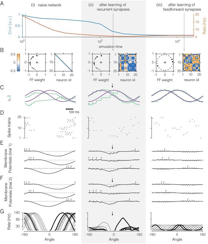
Fig 2. A 20-neuron network that learns to encode two randomly varying signals.

A. Evolution of coding error (blue), defined as the mean-square error between input signal and signal estimate, and mean population firing rate (orange) over learning. B. Feedforward and recurrent connectivity at three stages of learning. In each column, the left panel shows the two feedforward weights of each neuron as a dot in a two-dimensional space, and the right panel shows the matrix of recurrent weights. Here, off-diagonal elements correspond to synaptic weights (initially set to zero), and diagonal elements correspond to the neurons’ self-resets after a spike (initially set to -0.5). C. Time-varying test input signals (purple) and signal estimates (green). The test signals are a sine wave and a cosine wave. Signal estimates in the naive network are constructed using an optimal linear decoder. Arrows indicate parts of the signal space that remain poorly represented, even after learning of the recurrent weights. D. Spike rasters from the network. E. Voltages and spike times of three exemplary neurons (see thick dots in panel B). Dashed lines illustrate the resting potential. Over the course of learning, voltage traces become confined around the resting potential. F. As in E, but for a different trial. G. Tuning curves (firing rates as a function of the angle of an input signal with constant radius in polar coordinates for all neurons in the network. Angles from −90° to 90° correspond to positive values of x₁ which are initially not represented (panel B).