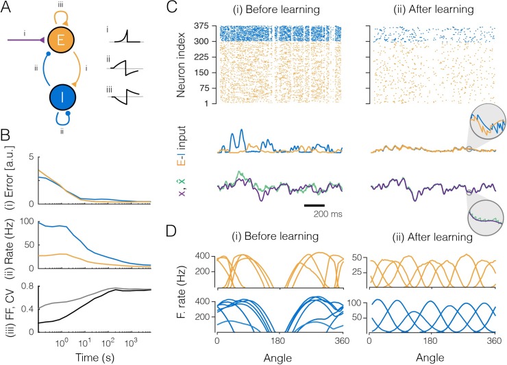
Fig 4. Large network (300 excitatory and 75 inhibitory neurons) that learns to encode three input signals.

Excitation shown in orange, inhibition in blue. A. The EI network as in Fig 1Ai and the learning rules (i, feedforward rule; ii and iii, recurrent rule). The insets show cartoon illustrations of the learning rules, stemming from STDP-like protocols between pairs of neurons, with the x-axis representing the relative timing between pre- and postsynaptic spikes (Δt = t_pre−t_post), and the y-axis the change in (absolute) weight. Note that increases (decreases) in synaptic weights in the learning rules map onto increases (decreases) for excitatory weights and decreases (increases) for inhibitory weights. This sign flip explains why the STDP-like protocol for EE connections yields a mirrored curve. B. Evolution of the network during learning. (i) Coding error for excitatory and inhibitory populations. The coding error is here computed as the mean square error between the input signals and the signal estimates, as reconstructed from the spike trains of either the excitatory or the inhibitory population. (ii) Mean firing rate of excitatory and inhibitory populations. (iii) Averaged coefficient of variation (CV, gray) and Fano factor (FF, black) of the spike trains. C. Network input and output before (i) and after (ii) learning. (Top) Raster plots of spike trains from excitatory and inhibitory populations. (Center) Excitatory and inhibitory currents into one example neuron. After learning, inhibitory currents tightly balance excitatory currents (inset). (Bottom) One of the three input signals (purple) and the corresponding signal estimate (green) from the excitatory population. D. Tuning curves (firing rates as a function of the angle for two of the input signals, with the third signal clamped to zero) of the most active excitatory and inhibitory neurons.