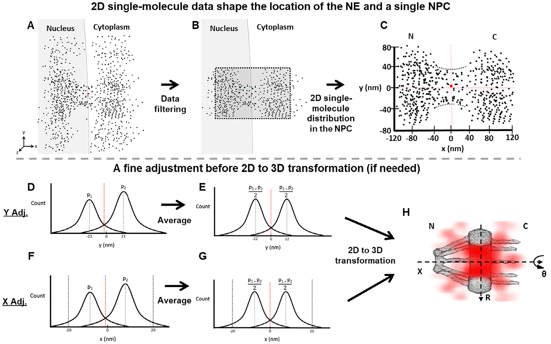
Fig. 2.

Determination of the central axis of the NPC illuminated by SPEED microscopy. Diagrams are used to demonstrate the detailed steps in our data analyses. (A) The initial single-molecule tracking data (black points) are plotted around the NPC’s marker (red dot) collected with SPEED. (B) The collected data after filtering by using single-molecule spatial localization precision. (C) The filtered 2D single-molecule data shape the spatial location of the NE and a single NPC. The red dot represents the location of the NPC’s marker. But sometimes the marker’s position is not perfectly overlapped with the averaged central positions in either x or y dimension suggested by the 2D single-molecule data. Also, the 2D single-molecule distribution also indicates the orientation of NPC. If the orientation of the NPC is within a free angle of 1.4° to the perpendicular direction to the NE [51], the 2D single-molecule data will be proceeded further. If it is bigger, the data will be dropped. (D) The plot of projected locations of these 2D single-molecule data in the y dimension will indicate if a fine adjustment for the central cytoplasmic transport axis is needed or not. Here we just show an example that peak 1 (p1) and peak 2 (p2) are not symmetrical locating at −23 nm and 21 nm respectively. If the peaks are symmetrical, the step E will be skipped to move onto the 2D to 3D transformation directly. (E) The two peaks are averaged as , resulting a fine adjustment in the NPC’s central cytoplasmic transport axis. The dotted red line has shifted to the corrected central position. (F and G) Similar to the y-dimensional data process, we next determine the precise location of the NPC’s central position along the x dimension by fitting the histogram of these 2D single-molecule locations within the NPC’s scaffold region projected into the x dimension (ranging from −20 nm to 20 nm, as clearly shown in the void region of the NE in (C) even if the NPC’s marker is a little bit off sometimes). (H) The 2D single-molecule data with the confirmed x and y axes will undergo the 2D to 3D transformation (Fig. 3) to produce the 3D density map of mRNP’s nuclear export routes (red clouds).
