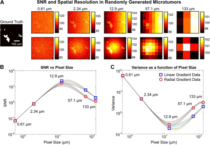
Figure 6.

Monte Carlo simulation of procedurally generated tumor images. A, Example of randomly generated tumor followed by images at various spatial resolutions with simulated noise. The average background and noise are modeled after empirically determined distributions. The top and bottom row illustrate a linear and radial low-frequency noise gradient, respectively. B, Plot of signal to noise ratio (SNR) at various pixel sizes over 20 randomly generated tumors. Ten were simulated with linear low-frequency noise, where the blue squares indicate the data for the images in the top row of part (A). Ten were simulated with radial low-frequency noise, where the red circles indicate data for the bottom row in part (A). C, Variance across an image at various pixel sizes. Variance decreases as high-frequency noise is averaged away and then increases as low-frequency noise dominates.