Figure 3. Bistability may favor survival of populations with highest or lowest initial density.

(A) Main panel: phase diagram indicating regions of extinction (black), survival (white), bistability (light gray; initially large population survives, small population dies), and ‘inverted’ bistability (dark gray; initially small population survives, large population dies). Red ’x’ marks correspond to the subplots in the top panels. Top panels: time-dependent population sizes starting from a small population (OD = 0.1, blue) and large population (OD = 0.6, red) at constant drug influx of $F_{\mathrm{2}}\mathrm{\gg }{F}_c$ (large drug influx) and $F_{\mathrm{1}}\mathrm{>}{F}_c$ (small drug influx). $F_c$ is the critical influx rate above which the extinct solution (population size 0) first becomes stable; it depends on model parameters, including media refresh rate (µ), maximum kill rate of the antibiotic ($g_{m\mathrm{}i\mathrm{}n}$), the Hill coefficient of the dose response curve ($h$), and the MIC of the drug-resistant population in the low-density limit where cooperation is negligible ($K$). Specific numerical plots were calculated with $h\mathrm{=}\mathrm{1.4}$, $g_{m\mathrm{}i\mathrm{}n}\mathrm{=}\mathrm{1}\mathrm{/}\mathrm{3}$, $g_{m\mathrm{}a\mathrm{}x}\mathrm{=}\mathrm{1}$, ${ϵ}_{\mathrm{1}}\mathrm{=}\mathrm{1.1}$, ${ϵ}_{\mathrm{2}}\mathrm{=}\mathrm{1.5}$, $\gamma \mathrm{=}\mathrm{0.1}$, $K_r\mathrm{=}\mathrm{14}$, $F_{\mathrm{1}}\mathrm{=}\mathrm{1.4}$, and $F_{\mathrm{2}}\mathrm{=}\mathrm{2.2}$. (B) Experimental time series for mixed populations starting at a total density of OD = 0.1 (blue) or OD = 0.6 (red). The initial populations are comprised of resistant cells at a total population fraction of 0.2 (left), 0.55 (center), and 0.80 right) for influx rate $F_{\mathrm{1}}\mathrm{=}\mathrm{650}$ µg/mL. Light curves are individual experiments, dark curves are means across all experiments. (C) Experimental time series for mixed populations starting at a total density of OD = 0.1 (blue) or OD = 0.6 (red). The initial populations are comprised of resistant cells at a total population fraction of 0.02 (left), 0.11 (center), and 0.35 right) for influx rate $F_{\mathrm{1}}\mathrm{=}\mathrm{18}$ µg/mL. Light curves are individual experiments, dark curves are means across all experiments.

Figure 3—figure supplement 1. Alternative mathematical models exhibit similar qualitative features, including inverted bistability.

Phase diagrams indicating regions of extinction (black), survival (white), bistability (light gray; initially large population survives, small population dies), and ‘inverted’ bistability (dark gray; initially small population survives, large population dies). Specific numerical plots were calculated with $h=3$, $g_{min}=1/3$, $g_{max}=1$, ${ϵ}_1=1.1$, ${ϵ}_2=1.5$, $\gamma =0.1$, and $K_r=14$. In the enzyme release model, simulations were run with $\chi =0.1$ (lysed cells degrade drug at 0.1 times the rate of living cells). For simplicity, we also choose $ep{s}_3=1$ in the pH-IC₅₀ model and $c_0=1$ in the Monod growth model.

Figure 3—figure supplement 2. Time series of cell density for simulations starting from high- or low-density populations in Monod growth model.

Time series of cell density for populations starting from a density of 0.6 (red) or 0.1 (blue) for different values of the drug influx rate (different rows) and initial resistant fractions (different columns). Column headings indicate initial resistant fraction; row headings on right indicate drug influx rate. Specific numerical plots were calculated with $h=3$, $g_{min}=1/3$, $g_{max}=1$, ${ϵ}_1=1.1$, ${ϵ}_2=1.5$, $\gamma =0.1$, and $K_r=14$. Background color indicates that both populations go extinct (red), both populations survive (white), high-density populations survive while low-density populations go extinct (dark blue; bistable), or high-density populations die while low-density populations survive (green; ‘inverted bistable’).

Figure 3—figure supplement 3. Short experiments to explore parameter space for inverted bistability.

Cell density (OD) time series at various initial resistant fractions (columns) and ampicillin influx rate (rows). Populations were started at OD = 0.1 (blue curves) or OD = 0.6 (red curves). Red shaded plots indicate both populations are near extinction, while green shaded plots indicate that both populations are near carrying capacity at end of experiment (<5 hr).

Figure 3—figure supplement 4. Time series of cell density for simulations starting from high- or low-density populations in enzyme release model.

Time series of cell density for populations starting from a density of 0.6 (red) or 0.1 (blue) for different values of the drug influx rate (different rows) and initial resistant fractions (different columns). Column headings indicate initial resistant fraction; row headings on right indicate drug influx rate. Specific numerical plots were calculated with $h=3$, $g_{min}=1/3$, $g_{max}=1$, ${ϵ}_1=1.1$, ${ϵ}_2=1.5$, $\gamma =0.1$, $\chi =0.1$, and $K_r=14$. Background color indicates that both populations go extinct (red), both populations survive (white), high-density populations survive while low-density populations go extinct (dark blue; bistable), or high-density populations die while low-density populations survive (green; ‘inverted bistable’).

Figure 3—figure supplement 5. Time series of cell density for simulations starting from high- or low-density populations in pH-IC₅₀ model.

Time series of cell density for populations starting from a density of 0.6 (red) or 0.1 (blue) for different values of the drug influx rate (different rows) and initial resistant fractions (different columns). Column headings indicate initial resistant fraction; row headings on right indicate drug influx rate. Specific numerical plots were calculated with $h=3$, $g_{min}=1/3$, $g_{max}=1$, ${ϵ}_2=1.5$, ${ϵ}_3=1$, $\gamma =0.1$, and $K_r=14$. Background color indicates that both populations go extinct (red), both populations survive (white), high-density populations survive while low-density populations go extinct (dark blue; bistable), or high-density populations die while low-density populations survive (green; ‘inverted bistable’).

Figure 3—figure supplement 6. Time series of cell density for simulations starting from high or low-density populations.

Time series of cell density for populations starting from a density of 0.6 (red) or 0.1 (blue) for different values of the drug influx rate (different rows) and initial resistant fractions (different columns). Column headings indicate initial resistant fraction; row headings on right indicate drug influx rate. Specific numerical plots were calculated with $h=3$, $g_{min}=1/3$, $g_{max}=1$, ${ϵ}_1=1.1$, ${ϵ}_2=1.5$, $\gamma =0.1$, and $K_r=14$. Background color indicates that both populations go extinct (red), both populations survive (white), high-density populations survive while low density populations go extinct (dark blue; bistable), or high-density populations die while low-density populations survive (green; ‘inverted bistable’).

Figure 3—figure supplement 7. Isolates from populations exhibiting collapse but not complete extinction show similar dose-response behavior as original strains.

Dose response curves illustrate effect of AMP on final cell density (left) and per capita growth rate (right). Bold curves correspond to original sensitive (blue) and resistant (red) strains. Light curves correspond to randomly selected single-colony isolates taken from collapse populations (11% initial resistant fraction; drug influx rate of 18 g/mL; initial density of 0.6; see Figure 3C, middle panel, red curves) at the end of the experiment. Points are mean ± 1 SEM over three technical replicates.

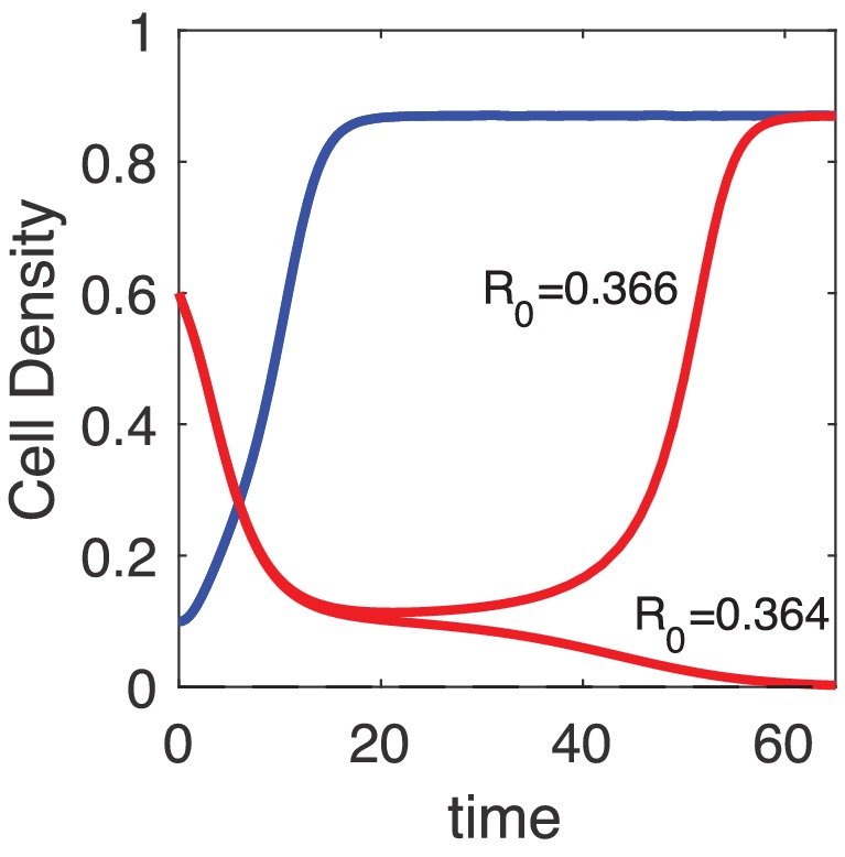
Figure 3—figure supplement 8. Populations exhibit transient periods of approximately constant density near regions of inverted bistability.

Populations starting from a density of 0.6 collapse and exhibit long-lived states of nonzero, nearly-constant density on timescales comparable to or longer than those at which low-density populations reach steady state (in this example, approximately 10 hr). These transient long-lived states ultimately collapse or recover, depending on the specific value of $R_0$ (the initial resistant fraction).