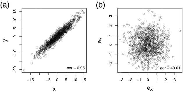
Figure 1: Scatterplots before and after variable adjustment.

Figure (a) shows the scatterplot of 1000 measurements between two multivariate normal random variables X and Y. Figure (b) takes into account the effect of a third random variable Z, which is associated with both X and Y. Here, we calculated the residues e_X and e_Y after a linear regression of X with Z and of Y with Z. We observe that the correlation between X and Y in (a) can be entirely explained by variable Z as shown in Figure (b). The corresponding Pearson correlation coefficients are given in the lower right corners. Data were simulated from a three-dimensional multivariate normal distribution, (X, Y, Z)^T ~ N(0, Ω⁻¹), where the precision matrix Ω is defined by ω₁₁ = ω₂₂ = ω₃₃ = 1, ω₃₁ = ω₃₂ = ω₁₃ = ω₂₃ = −0.7 and 0 elsewhere, as outlined in the Supplementary File 1.