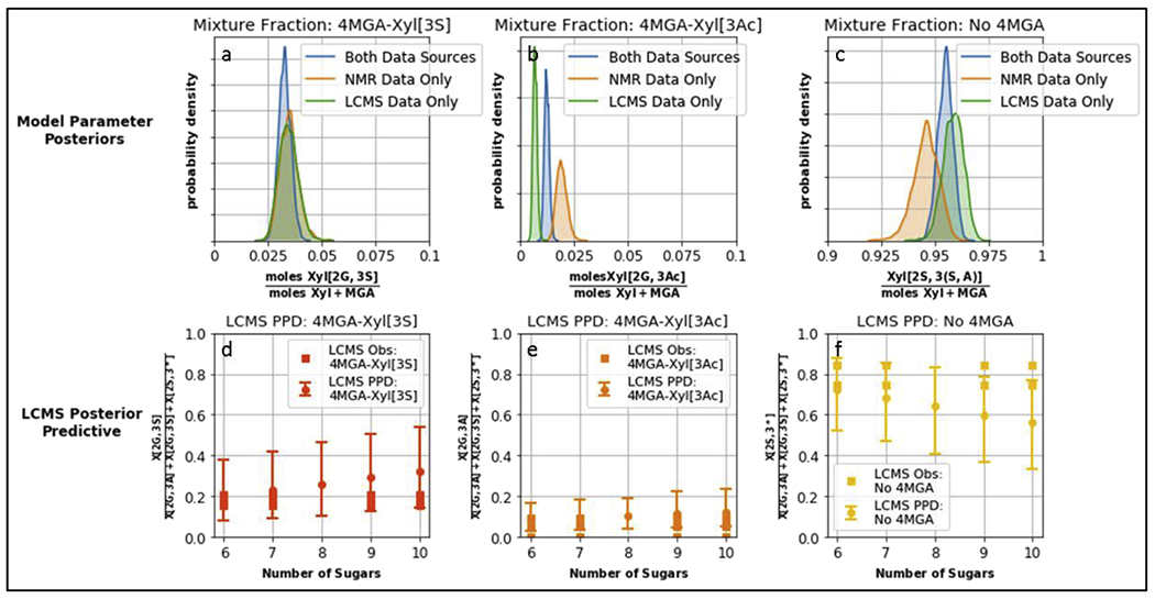
Fig.4.

Top row: posterior distribution of building block fractions Xyl[2G,3S], Xyl[2G, 3Ac], Xyl[2S, 3(S,A)], as estimated when using either one or both of the data sources. Width of the distribution indicates the variability in estimating the parameter. Bottom row: the model provides a posterior predictive distribution for the LC-MS measurements, plotted with 90% credible intervals. An advantage of using a Bayesian framework is that we can simulate the distribution of measurement values in addition to the unobserved parameter values. Note that the credible intervals in panels d,e,f incorporate both the parameter variability shown in figures a,b,c respectively as well as a component of measurement variability.
