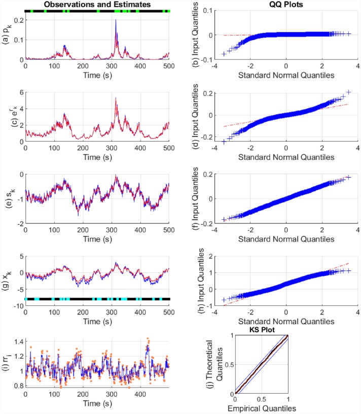
Fig 6. State estimation with simulated data (${\widehat{p}}_0>0.01$).

The sub-panels respectively depict, (a) the Bernoulli trial probabilities p_k (blue), their estimate (red) and the presence or absence of binary observations (light green and black dots); (b) the quantile-quantile (QQ) plot for the residual error of p_k; (c) the exponent of r_k (blue) and its estimate (red); (d) the QQ plot for the residual error of r_k; (e) s_k (blue) and its estimate (red); (f) the QQ plot for the residual error of s_k; (g) the arousal state x_k (blue), its estimate (red) and the presence or absence of stimuli I_k driving the state (cyan and blacks dots); (h) the QQ plot for the residual error of x_k; (i) the sequence of RR-intervals rr_i (orange dots) and the estimated RR-interval mean μ (solid blue line); (j) the KS plot for the heartbeats.