Fig. 4.

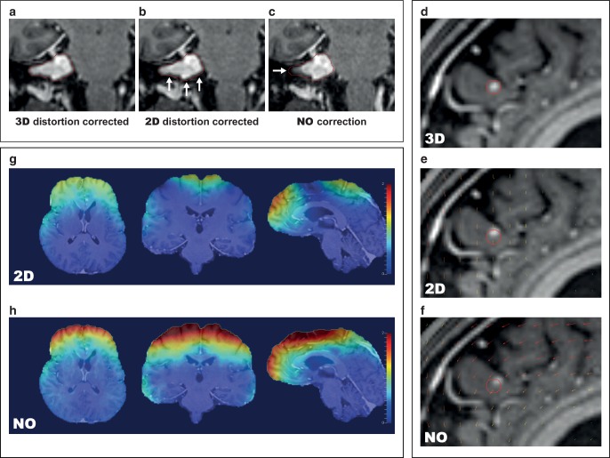
Impact of gradient nonlinearity distortion correction. a–c Example of a case with vestibular schwannoma. Comparison of vendor-specific 3D- (a) and 2D-distortion correction (b) with the uncorrected T1-MPRAGE dataset (c). Tumor outline (red) from the 3D-corrected dataset is projected onto the 2D-corrected and uncorrected dataset for reference. Note: While the difference between 2D- and 3D-correction is more subtle, the 2D-corrected dataset underestimates the lower border of the tumor (white arrows). d Example in a patient with a prefrontal brain metastasis. Sagittal view. The tumor is significantly displaced in the uncorrected (f) and 2D-corrected dataset (e). Arrows indicate the amount of tissue distortion in the 2D- and uncorrected images with reference to the 3D-corrected dataset. Note: The 2D-corrected dataset contains residual through-plane distortions. g, h Amount of displacement with reference to 3D-corrected images overlaid as heatmap. Blue indicates no displacement, red indicates a displacement of 2 mm. While 2D-corrected images (g) show fewer residual distortions than uncorrected images (h), distortions of up to 2 mm were still present after 2D-correction. Note: The amount of gradient nonlinearity-related distortions for other scanner models and patient positions is different from the examples shown here. Additional sources of distortion include magnet imperfections and patient-induced susceptibility-related distortions, which are not visualized here