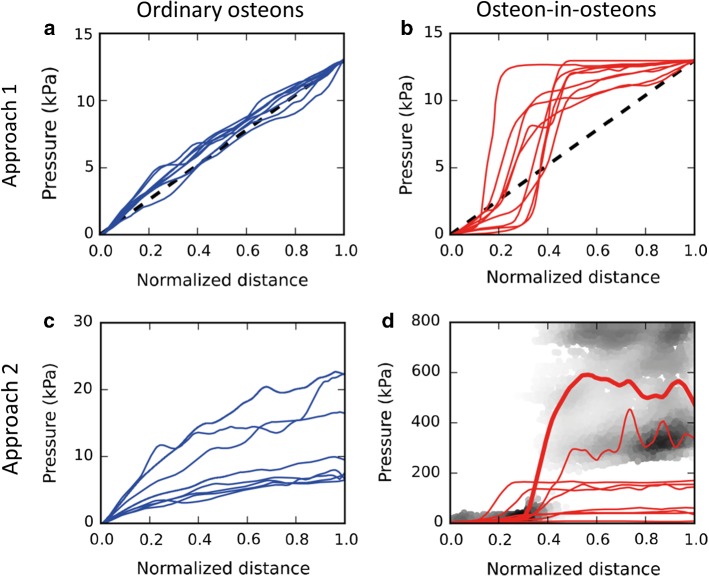
Fig. 4.

Pressure profiles plotted as a function of the normalized distance (Haversian canal = 0, cement line = 1). The profiles were obtained, firstly, by presenting for each node the values of its position (given by a value between 0 and 1 as normalized distance) and its pressure. Secondly, the data of all nodes in this scatter plot (plot not shown) were transformed in the shown profiles by using a local regression algorithm (locally weighted scatterplot smoothing, LOWESS). a and c Show the pressure profile for all 8 ordinary osteons; b and d show pressure profiles for all 9 osteon-in-osteons. In a and b the dashed line serves as a reference of a linear decrease of the applied pressure. In the background of d the gray values indicate the density of data points of the scatter plot for the osteon-in-osteon of Fig. 3d. The corresponding LOWESS fit is shown by the thicker red line. This kind of representation was chosen to highlight the spatial heterogeneity of the pressure distribution in this case, which can be only poorly rendered by a LOWESS fit