Fig. 4.

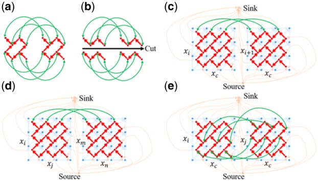
Construction of the various GTW graphs used in the different steps of ncGTW algorithm (Wang et al., 2016). (a) Two small DTW graphs are linked to form a GTW graph via additional ‘connecting’ edges (green lines between the vertices as the same position of two DTW graphs). (b) After adding the green edges, we can solve all warping functions at the same time, with the similarity among warping functions as constraints. The cost on green edges is to control the similarity between warping functions. For example, if the cost is very high, no green edge will be cut and all the warping functions would be the same. (c) GTW graph formed by two linked DTW graphs of two neighboring samples (x_i and x_(i+1)) with a common reference, extendable to all neighboring samples, where the orange lines link vertices to a single source or sink forming a large maximum flow graph, while green edges link the corresponding vertices of two DTW graphs (only edges linking top three vertices are shown here). (d) Part of the graph constructed in Stage 1 of ncGTW without using a common reference, where x_i and x_m are neighboring samples, and x_j and x_n are neighboring samples. (e) Part of the graph constructed in Stage 2 based on all pairwise warping functions obtained in Stage 1, where the warping function Φ_(i→j) guides the links between the corresponding vertices in GTW graphs, with x_c being the virtual reference. (Color version of this figure is available at Bioinformatics online.)