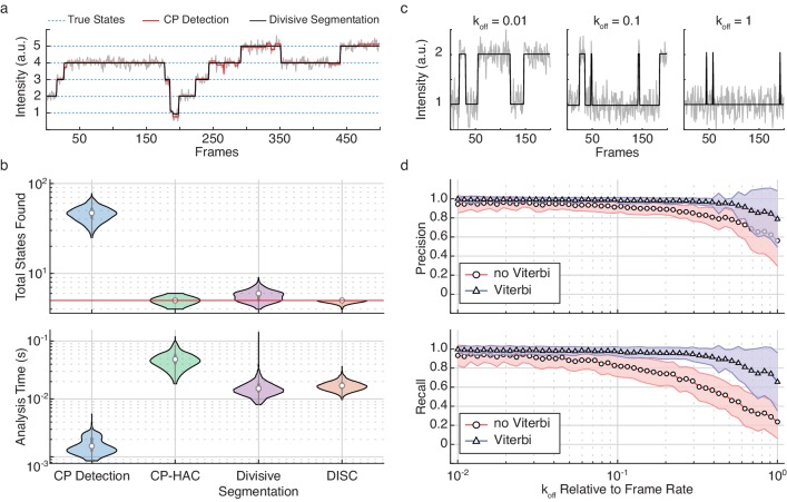
Figure 2. Refinement of divisive segmentation.

(a) Example trajectory simulated with five states (blue) at a SNR = 5 overlaid with fits obtained from change-point detection (red) and divisive segmentation (black). (b) Violin plots showing the number of identified states (top) and analysis time (bottom) of each algorithm across 500 simulated trajectories featuring five true states (red line). (c) Example simulations of a two-state system with a k_on = 0.02 frames⁻¹ and varying k_off. (d) Precision (top) and recall (bottom) values obtained with CP detection (no Viterbi) and Viterbi refinement obtained across 100 trajectories per k_off (mean ± s.d.).

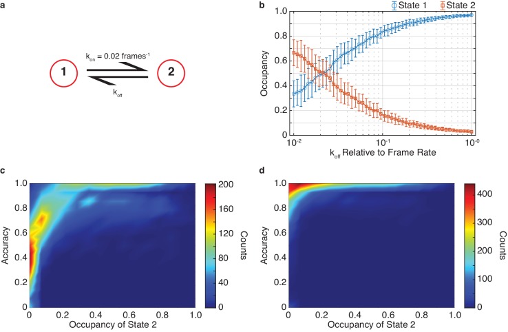
Figure 2—figure supplement 1. The effect of state occupancy on DISC.

(a) Simulated kinetic scheme of Figure 2 featuring two states with a constant k_on (k_on = 0.02 frames⁻¹) and varying k_off. (b) Occupancy of state 1 (blue circles) and state 2 (orange squares) for different simulated k_off values (mean ± s.d.). (c, d) Density plot of idealization accuracy per trajectory vs the occupancy of state two across all simulations (N = 5000) for results obtained without (c) and with Viterbi refinement (d).