Fig. 1.

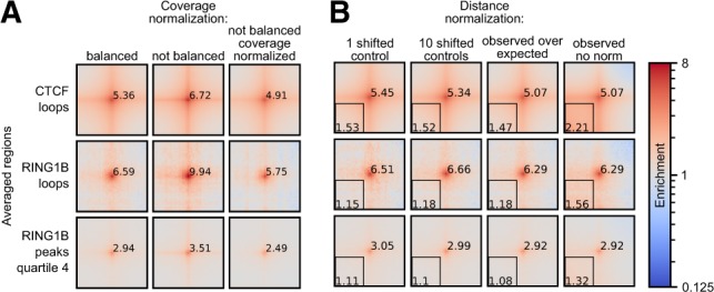
Hi-C data normalization strategies. (A) Comparison of coverage normalization strategies for pile-up analyses using mouse ES cell Hi-C data (Bonev et al., 2017). Normalization approaches are in columns: matrix balancing (iterative correction); no normalization; no balancing with coverage normalization of the pile-ups. The different averaged regions are shown in rows: loops associated with CTCF (n = 6536), loops associated with RING1B (n = 104) (see Materials and Methods section), all pairwise combinations of high RING1B peak regions from the fourth quartile (by RING1B ChIP-seq read count) (n = 2660 of peak regions). All pile-ups produced with 10 randomly shifted controls. All pile-ups are normalized to the average of the top-left and bottom-right corner pixels to bring them to same scale. Value of the central pixel is displayed. Five kilobytes resolution with 100 kb padding around the central pixel. Colour is shown in log-scale and shows enrichment of interactions. (B) Same as (A), but for different approaches to remove distance-dependency of contact probability with balanced data. In columns: single randomly shifted control regions per ROI; 10 randomly shifted control per ROI; normalization to chromosome-wide expected; no normalization. Same rows as in (A). Average enrichment of the lower-left corner of the pile-up is displayed