
Figure 11.
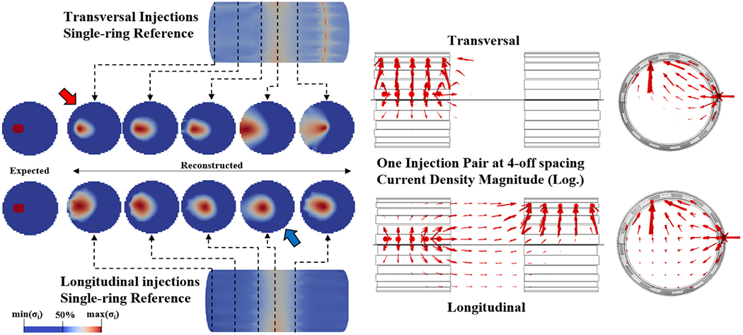
Left: Visual comparison of reconstructed conductivity changes along different x-axis locations for one example perturbation with TS/LS configurations and 4-off spacing. Each slice is shown with FWHM colour scheme for its own value range. Red and blue arrows identify optimal reconstruction location for TS and LS protocols, respectively. Right: arrows representing logarithm of current density in the reconstructed volume for one example injection pair at 4-off spacing in transversal and longitudinal configurations.