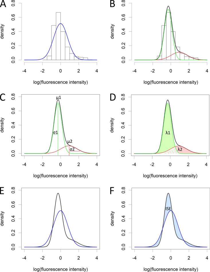
FIG 3.

Level of heterogeneity explained. (A) First, the data are log transformed to reduce skewedness. Even after log transformation, the data (histogram) cannot be fitted with a single normal distribution (blue line). (B) Using the Bayesian information criterion (BIC) (see Materials and Methods) the number of subpopulations is determined. This calculation penalizes for adding additional subpopulations. In this study, all data could always be described by two subpopulations. The data are then fitted with a mixture of two normal distributions. Subpopulation 1 is indicated by a green line, subpopulation 2 by a red line, and the total fit, which is the sum of the two normal distributions is depicted with a black line. This fit can be described using three parameters: μ, σ (C), and λ (D) of each subpopulation, that represent the mean, standard deviation, and proportion of each subpopulation to the total population of cells, respectively. The area under each subpopulation fit is λ_n (λ₁ green and λ₂ pink shaded areas under the curves in panel D). λ₁ + λ₂ = 1, since the sum represents the total population. (E) If we now plot the theoretical normal distribution from panel A (blue line) and the mixture normal distribution from panel B (black line), we can calculate the integrated squared error (ISE) (F) using μ, σ, and λ of each subpopulation (see Materials and Methods), which is basically the squared error of the surface area difference between the two lines (blue shaded areas between the curves) and indicates the level of heterogeneity. The data used to produce this figure are CFW-stained dormant conidia of strain CEA10 that had been grown for 3 days on minimal medium (MM) after spot inoculation to produce a radially extending colony.