Fig. 2.

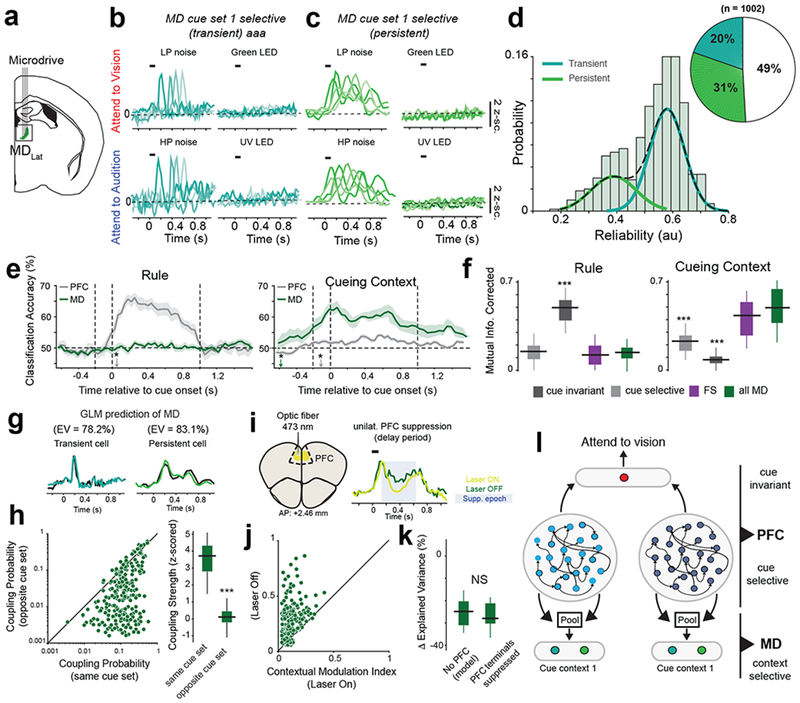
Mediodorsal thalamic responses reflect the cueing context.

(a) Schematic for MD recordings. (b-c) Example PSTHs of MD neurons with transient (b) and persistent (c) responses to both cues within the auditory cueing context. Each color indicates a distinct neuron. Representative examples drawn from n = 5 mice (independent samples). (d) Histogram of inter-trial spiking reliability scores from all task-modulated MD neurons. A gaussian mixture model (dashed lines) was used to classify cells into either persistent (low reliability) or transient (high reliability). Inset, pie chart quantifying the fraction of each MD neuron type. (e) Classification accuracy over time relative to cue onset for a decoder trained to predict either rule (top) or cue context decoding (bottom)trained to classify rule (left) and cue context (right) from PFC RS and MD populations (5 mice). The asterisks denote the time point at which classification accuracy is significant (i.e. p < 0.05, permutation test from n = 5 biologically-independent mice) above chance (50% classification accuracy). (f) Comparison of rule decoding and cueing context decoding accuracy, measured as mutual information (see Methods), between all recorded cell types. ***p < 0.001 Bonferroni-corrected Kruskal-Wallis ANOVA with post-hoc rank-sum test relative to MD neurons (n = 5 biologically-independent mice). (g) Generalized linear model (GLM) of MD neurons can accurately predict the responses of both transient (right) and persistent cells (left). EV, explained variance. Data: black, prediction: colored lines. (h) Left: Comparison of coupling probability between PFC cue-selective neurons and MD neurons within the same cue set and the opposite cue set. Right: Box-plot comparing coupling strength between MD and PFC cells selective to cues in the same cue context or the opposite context. *** p = 0.15 x 10⁻⁴ Bonferroni-corrected Kruskal-Wallis test (n = 345 MD neurons, 5 mice). (i) Left: Schematic illustrating unilateral PFC suppression. Right: Example MD neuron with suppressed firing rate following PFC suppression. Shaded blue area marks time over which the laser was turned on. (j) Comparison of contextual modulation index on Laser ON and Laser OFF trials. (k) Change in GLM prediction, measured as Δ Explained Variance, when PFC filters are excluded from the model (“No PFC”) compared to a model fit to MD responses following PFC suppression. Non-significant (NS, p = 0.42), Bonferroni-corrected Kruskal-Wallis test, n = 186 MD neurons, 3 mice. (l) Schematic of proposed PFC-MD connectivity. Data in d-h is from 5 mice, data in j,k is from 3 mice. Data is shown as mean +/− 95% confidence interval (shaded error-bars). Box plots: median (line), box edges, 95% confidence interval, whiskers, range.