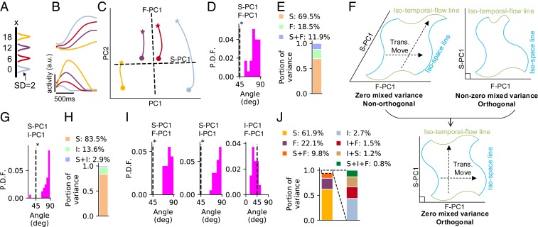
Fig. 3.

The t-SR task. (A) Color scheme that represents the spatial location of the first pulse used in B and C. Location is represented by Gaussian bump with SD of 2. (B) Firing profiles of four example neurons in the perception epoch. (C) Trajectory of the perception epoch in the subspace of the first two PCs. Stars indicate the points after 400 ms of the transient period from the beginning of the perception epoch, and circles indicate the ending points of the perception epoch. Dashed lines represent the projections of F-PC1 and S-PC1 in this subspace. (D) Probability distribution function (P.D.F.) of the angle between F-PC1 and S-PC1 in the perception epoch over 32 training configurations. *Significant ($P<0.05$) larger than $45^{○}$ (t test). (E) Portion of variance explained by spatial information (S), temporal flow (F), and their mixture (S + F) in the perception epoch, averaging over 32 training configurations. (F) Schematic for the meanings of angle and mixed variance. Zero mixed variance implies that different isospace (blue) or isotemporal flow (green) lines are related by translational movement, forming parallelogram-like grids (F, Upper Left); orthogonality (F, Upper Right) implies rectangle-like grids (F, Lower). (G) The distribution of the angle between I-PC1 and S-PC1 in manifold $\mathcal{M}$ (Fig. 2E) at the end of the delay epoch. (H) The portion of variance explained by S, time interval (I), and their mixture (S + I) in manifold $\mathcal{M}$ at the end of the delay epoch. (I) The distributions of the angles between F-PC1, I-PC1, and S-PC1 in the production epoch. (J) The portion of variance explained by S, F, I, and their mixtures in the production epoch. In A–E, $T=\mathrm{1,200}$ ms for the perception epoch; in G–J, $T=600$, 700$\cdots \hspace{0.17em}$1,200 ms for the delay and production epochs.