
Figure 8.
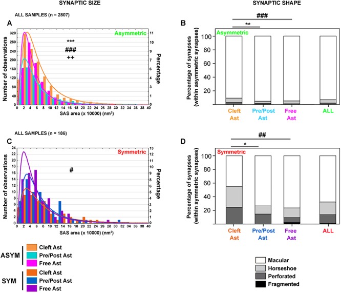
Synaptic size and shape of synapses classified according to their contacts with labeled astrocytic compartments. A, Frequency distribution histogram of SAS areas of asymmetric synapses classified according to their 3D contact with the labeled astrocytic compartments in all samples. Larger SAS areas were more frequently found within the population of asymmetric “Cleft Ast synapses” when compared with “Pre/Post Ast synapses” (KS, P = 0.000, ***) and “Free Ast synapses” (KS, P = 0.000, ###). Larger SAS areas were also more frequently found within the population of “Pre/Post Ast synapses” when compared with “Free Ast synapses” (KS, P = 0.003, ++). B, Proportion of macular (white), horseshoe (light gray), perforated (dark gray) and fragmented (black) asymmetric synapses classified according to their 3D contact with the labeled astrocytic processes and for all asymmetric synapses. “Cleft Ast synapses” had a higher proportion of synapses showing more complex shapes—horseshoe, perforated, and fragmented—when compared with “Pre/Post Ast” and “Free Ast synapses” (χ2, P = 0.002, ** and P = 0.001, ### respectively). C, Frequency distribution histogram of SAS areas of symmetric synapses classified according to their 3D contact with the labeled astrocytic compartments in all samples. Larger SAS areas were most frequently found within the population of symmetric “Cleft Ast synapses” when compared with “Free Ast synapses” (KS, P = 0.016, #). D, Proportion of macular (white), horseshoe (light gray), perforated (dark gray), and fragmented (black) symmetric synapses classified according to their 3D contact with the labeled astrocytic compartments and for all symmetric synapses. “Cleft Ast synapses” had a higher proportion of synapses showing more complex shapes—horseshoe, perforated, and fragmented—when compared with “Pre/Post Ast” and “Free Ast synapses” (χ2, P = 0.018, * and P = 0.006, ## respectively). In A, C, the log-normal function for each category has been represented. The x-axis bin = 2 (×10 000) nm2. See text and Supplementary Tables 6–8 for further details.