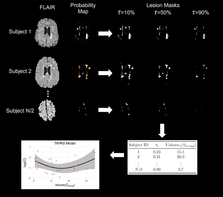
Figure 2.

The TAPAS procedure is shown using sample axial slices from the data. A set of training scans with manual delineations were used to train and apply MIMoSA in order to obtain probability maps. For each subject's probability map, we applied thresholds at $\tau =0\%$ to 100% by 1% to create estimated lesion masks. For simplicity, in this example, we have only shown $\tau =10\%$, 50%, and 90%. Based on Sørensen-Dice similarity coefficient (DSC) calculations within and across subjects we estimated ${\widehat{\tau }}_i$ and ${\widehat{\tau }}_{Group}$. Using ${\widehat{\tau }}_{Group}$ we obtained $volum{e}_i\left({\widehat{\tau }}_{Group}\right)$. We fit the TAPAS model and applied it to subjects in the test set to determine ${\widehat{\tau }}_i$. Red points in the plot represent ${\widehat{\tau }}^{0.1}$ and ${\widehat{\tau }}^{0.9}$, or lower and upper bounds at the volume associated with the 10th and 90th percentiles, respectively.