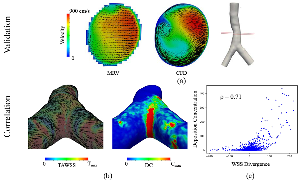
Figure 10:

Turbulent flow (Re=4500) simulation case. (a) Comparison of experimental MRV measurements versus CFD simulation results. The slice location at the trachea is shown in the figure and the corresponding velocity maps are colored based on velocity magnitude. Black vectors represent the secondary flow motion and the vector sizes correspond to the magnitude of secondary velocities. (b) The left panel is time-average WSS (TAWSS) vector colored by its magnitude rescaled to $T_{\mathit{max}}=5\frac{\mathit{dynes}}{{\mathit{cm}}^2}$ for visualization. The vectors are normalized to show the direction. The right panel displays the deposition concentration (DC), which is rescaled to C_max = 20. (c) Deposition concentration against WSS divergence (WSSdiv) scatter plot for d_p = 3μm is shown. DC is dimensionless and the WSSdiv unit is $\frac{\mathit{dynes}}{{\mathit{cm}}^3}$. Pearson’s correlation coefficient calculated for positive WSSdiv versus DC is 0.71.