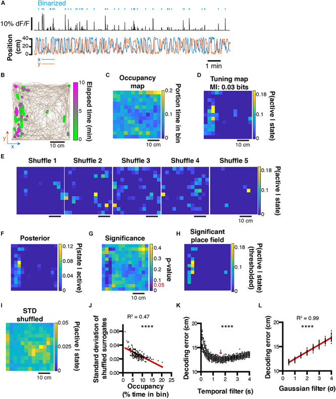
FIGURE 4.

Decoding two-dimensional behaviors. (A) x,y coordinates of mouse location in an open field (bottom) and corresponding raw calcium trace of one example cell and binarized activity (top). (B) Top view of mouse trajectory (beige trace) with overlaid location corresponding to neuronal activity (green, early activity; magenta, late activity). (C) Relative occupancy in the open field. (D) Tuning map (probability of being active given location) of one neuron. Top, corresponding MI index. (E) Example tuning maps computed from shuffled calcium traces. (F) Posterior probability P(state| active) for the same cell. (G) P-value computed from the actual tuning map and corresponding shuffled surrogates. (H) Thresholded place field using only significant P(active| state) values. (I) Standard-deviation of the shuffled distribution. (J) Scatter plot comparing the standard-deviation of the shuffled distribution, and the mouse open field occupancy. (K) Effect of temporal filtering on decoding error in the open field. The red arrow indicates the temporal filtering window size yielding the lower decoding error. (L) Effect of gaussian smoothing of tuning maps on decoding error in the open field.