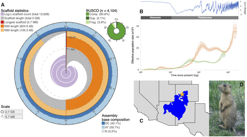
Fig. 1.

—(A) Assembly statistic visualization (https://github.com/rjchallis/assembly-stats) showing the genome N50 (dark orange), N90 (light orange), base composition (percentage of GC in dark blue, AT in light blue, and N in light grey), and BUSCO results (top right, in shades of green). (B) PSMC reconstruction of population size estimates over time, estimated using generation time of 2 years (g = 2) and two mutation rates: µ = 2.2 × 10⁻⁹ (green; “mammal rate”) and µ = 8.8 × 10⁻¹⁰ (orange; “Cynomys rate”). Shaded lines correspond to 100 bootstrap estimates. The ΔTemp (°C) was calculated using benthic d¹⁸O records (Lisiecki and Raymo 2005) and extrapolated using the formula from Epstein et al. (1953). (C) Map depicting the species distribution of C. gunnisoni (blue) in the western United States, with a star denoting the location where the sample was collected (Sackett et al. 2014). (D) Image of C. gunnisoni (LCS).