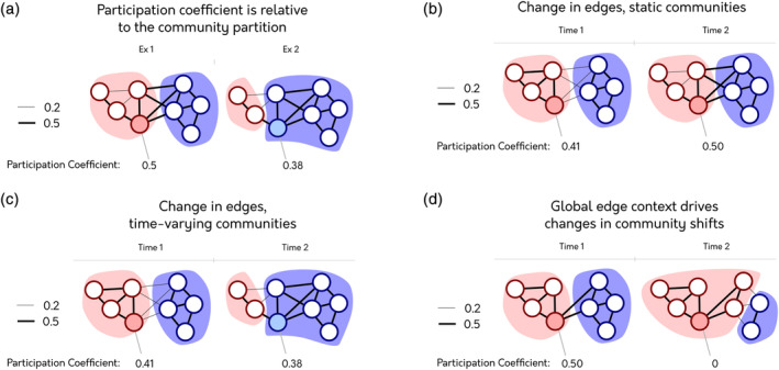
Figure 1.

Different ways to calculate the participation coefficient (PC) through time. The PC for the shaded node is below each network/temporal snapshot. The border of each node and the colored backgrounds show the assigned community of each node. In this example, there are two different possible edge weights. (a) Two examples of the PC, illustrating how the measure is calculated relative to the community partition. (b) An example of PC calculated when applying a static community template across multiple temporal snapshots (PC _S). (c) An example of PC calculated when applying a temporal community partition to multiple temporal snapshots (PC _T). PC values between time points cannot be directly compared due to differences in community structure obtained for each time point. (d) An example showing that changes in community partitions over snapshots may result from changes in edges that do not directly connect to the node of interest. The difference in community partition is the result of changes in the nodes in the blue community. These changes affect the PC of the shaded node despite the fact that there was no change in its connectivity