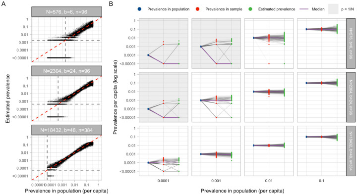
Fig. 3: Estimating prevalence from a small number of pooled tests.

In prevalence estimation, a total of N individuals are sampled and partitioned into b pools (with n=N/b samples per pool). The true prevalence in the entire population (x-axis in A) varies over time with epidemic spread. Population prevalences shown here are during the epidemic growth phase. (A) Estimated prevalence against true population prevalence using 100 independent trials sampling N individuals at each day of the epidemic. Each facet shows a different pooling design (more pooling designs shown in Fig. S1). Dashed grey lines show one divided by the sample size, N. (B) For a given true prevalence (x-axis, blue points), estimation error is introduced both through binomial sampling of positive samples (red points) and inference on the sampled viral loads (green points). Sampling variation is a bigger contributor at low prevalence and low sample sizes. When prevalence is less than one divided by N (grey boxes), inference is less accurate due to the high probability of sampling only negative individuals or inclusion of false positives.