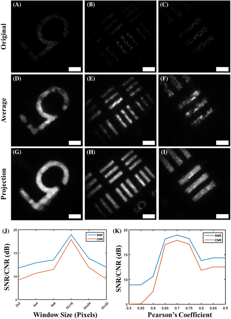
Fig. 3.

Comparison of the original and reconstructed images of features on a USAF resolution target. Three different locations are shown, one in each column. Results demonstrate the degree to which the algorithm is able to reveal object features that are otherwise obscured because of the superimposed fiber-pattern artifact, which is apparent in (A)–(C). More specifically, some regions do not appear in the original images, but can be seen after reconstruction [compare (B) and (E)]. Furthermore, regions with “dead” fibers, or fibers that do not transmit light, such as those seen in the number “5,” are effectively interpolated and show intensity after reconstruction [compare (A) and (D)]. These voids are more prominently filled when reconstruction involves taking the maximum value at each pixel between multiple images, as shown in (G)–(I). The image conditioning process for experimental data is optimized by selection of the optimal median window size (J) and inter-frame Pearson’s coefficient (K) that yields optimal image quality, as quantified using SNR and CNR. Scale bars represent 50 μm.