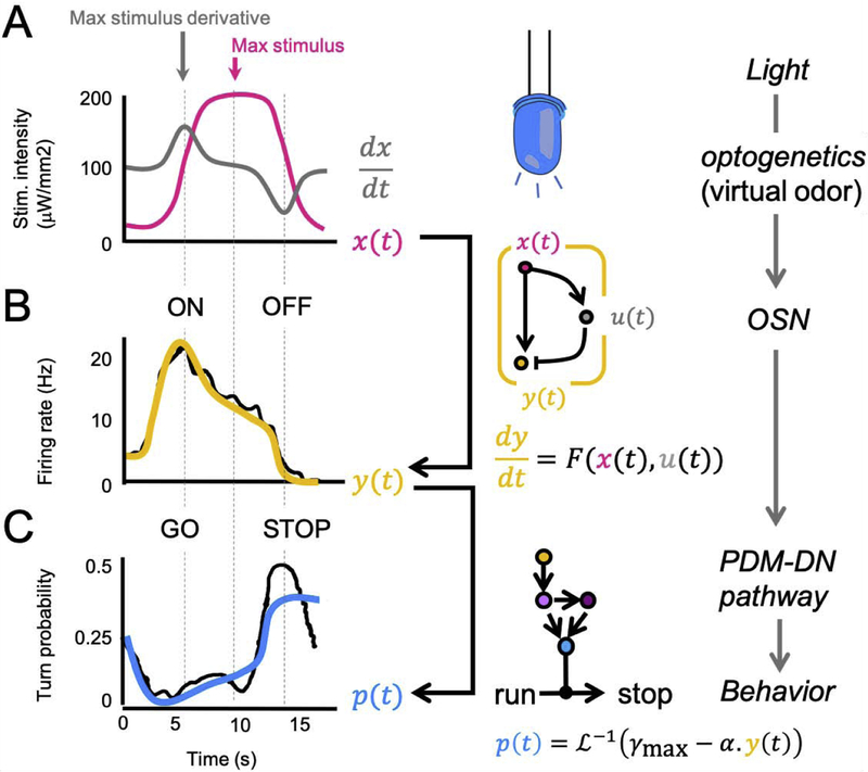
Figure 3: Computational model of the sensorimotor transformation that triggers the onset of reorientation maneuvers.

(A) Time course of a sigmoid ramp of light intensity (magenta) bearing resemblance with changes in stimulus experienced during real runs (Figure 1C). The temporal derivative of the ramp is shown in gray. (B) Peristimulus time histogram (PSTH) of the Or42a OSN expressing channel-rhodopsin (black trace) upon stimulation by the sigmoid light ramp shown in panel A. (Right) Coarse-grained biophysical model of the regulation of the firing activity of the Or42a OSN based on an incoherent feedforward motif (yellow diagram). The dynamics of the feedforward motif is described by an ordinary differential equation (ODE) that depends on the stimulus intensity (x(t)) and the activity state of an intermediate variable (u(t)). The molecular correlate of u remains to be determined [26]. The simulated dynamics of the ODE model is shown in yellow. (C) Time course of the instantaneous probability of implementing a transition from running to stopping (black trace). The probability is estimated over time bins of 1 s using a dataset of >500 runs paired with the same pattern of virtual-odor stimulation shown in panel 3A. (Bottom) Generalized linear model (GLM) of the sensorimotor transformation by the neural circuitry downstream from the Or42a OSN. The model predicts the probability of stopping. The linear part of the predictor combines a positive constant (γ_max) with the activity of the Or42a OSN (y(t)) multiplied by a positive constant (α). As a result, the linear predictor is equal to γ_max (max turn rate) when the activity of the OSN is suppressed during steep negative gradients whereas the linear predictor tends towards 0 (no turn) when the activity of the OSN is large during steep positive gradients. The function $L^{-1}$ is the inverse of the logit linker. The predicted behavior of the GLM is shown in blue in panel C. Data shown in panels A-C are redrawn from [26].