Highlights
-
•
Comparison of ARIMA, NARNN and LSTM models on COVID-19 prediction.
-
•
Detailed model performance criteria evaluation.
-
•
Prospective estimation of total cases with LSTM.
Keywords: COVID-19, Forecasting, ARIMA, NARNN, LSTM, Modeling
Abstract
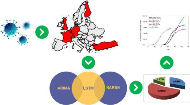
In this study, confirmed COVID-19 cases of Denmark, Belgium, Germany, France, United Kingdom, Finland, Switzerland and Turkey were modeled with Auto-Regressive Integrated Moving Average (ARIMA), Nonlinear Autoregression Neural Network (NARNN) and Long-Short Term Memory (LSTM) approaches. Six model performance metric were used to select the most accurate model (MSE, PSNR, RMSE, NRMSE, MAPE and SMAPE). According to the results of the first step of the study, LSTM was found the most accurate model. In the second stage of the study, LSTM model was provided to make predictions in a 14-day perspective that is yet to be known. Results of the second step of the study shows that the total cumulative case increase rate is expected to decrease slightly in many countries.
Graphical abstract
1. Introduction
The last epidemic process, which started on December 31, 2019 with the World Health Organization (WHO) China Country Office reporting cases of pneumonia of unknown etiology in Wuhan, China, continued with the identification of a new Coronavirus (2019-nCoV) and this new virus spread rapidly and became a global problem. The new virus-related disease is named COVID-19, while the virus is named SARS-CoV-2 because of its similarity to SARS CoV [1].
The rate of contagion and spread of infection is quite fast compared to other viral infections encountered until today. Due to its rapid progress and covering the world in a short period of time, it is necessary to carry out intensive studies in it. Similar to many other infectious disease outbreaks, the success of controlling the new COVID-19 infection is based on revealing significant information, especially in the early period, with very limited data. For this, it is necessary to monitor the cases correctly and increase the reliability of the future predictions with each new data [2].
There are many studies in the literature on the prediction of epidemic diseases. The Auto-Regressive Integrated Moving Average (ARIMA) approach is often used to predict time series. The reason it is used so widely is that it can obtain useful statistical properties. They are also very flexible as they can represent multiple different time series using different order parameters. The ARIMA approach has been used to predict many diseases such as Hemorrhagic Fever with Renal Syndrome (HFRS) [3], Brucellosis [4], Influenza [5] and COVID-19 [6]. The Nonlinear Autoregression Neural Network (NARNN) model is a technique that performs nonlinear regression through the neural network. This machine learning technique has been used to predict various outbreaks [7], [8], [9].
The LSTM technique is a model that extends RNN (Recurrent Neural Network) memory. Typically, repetitive neural networks have "short-term memory" because they use persistent prior knowledge for use in the existing neural network. Essentially, previous information is used in the current task [10]. Studies involving the use of LSTM in the prediction of infectious diseases are rather scarce. In a study by Chimmula and Zhang (2020), COVID-19 infection in Canada was estimated by LSTM [11]. In the study by Tomar and Gupta (2020), COVID-19 infection in India was analyzed and predicted with LSTM [12].
In this study, unlike other studies, the total number of cases in COVID-19 infection was modeled and estimated by ARIMA, NAR and LSTM approaches. The performance of the models examined has been compared. As a result of this comparative analysis, the most successful model was determined by considering six different performance parameters. At the same time, the data used in this study includes the widest time interval ever made. The data used includes 8 different European countries (Denmark, Belgium, Germany, France, United Kingdom, Finland, Switzerland and Turkey) where the disease progresses differently. After determining the most successful model, prospective forecasting study was carried out for the cumulative confirmed number of cases in each country.
2. Materials and methods
2.1. Data collection
In this study, cumulative confirmed case data of 8 different European countries (Denmark, Belgium, Germany, France, United Kingdom, Finland, Switzerland and Turley) were used for modeling. The data were obtained from European Center for Disease Prevention and Control [13]. Data were taken from the day the first case was seen, and the number of data for each country varies. The data covers 67, 90, 97, 100, 94, 90, 68 and 55 days respectively and ends on 3 May 2020. Dates of first recorded case of the investigated countries is given in Table 1 .
Table 1.
Dates of first recorded confirmed COVID-19 case for each investigated countries [13].
| Country | Date |
| Denmark | February 27, 2020 |
| Belgium | March 2, 2020 |
| Germany | January 28, 2020 |
| France | January 25, 2020 |
| United Kingdom | January 31, 2020 |
| Finland | January 39, 2020 |
| Switzerland | February 26, 2020 |
| Turkey | March 12, 2020⁎ |
Minor differences can be seen between the given dates and official announcements of related countries. All data were taken from official website of European Centre for Disease and Control.
2.2. ARIMA model
Auto Regressive Integrated Moving Average (ARIMA) technique is one of the commonly used approaches for time series investigation. The AR section of ARIMA model expresses that the evolving variable is regressed on its own prior values. In a stationary time series, the average of the error term is zero and the variance is expressed as σ 2. If Yt shows the value of the time series at time t, the expression of this time series as a p-order autoregressive process is as in Eq. (1) and shown as AR(p).
| (1) |
Here, δ is a constant value and ɛt is error term. Time series as a qth degree of moving average process MA(q) can be found as:
| (2) |
ARMA(p,q) expression can be obtained by combining two AR(p) and MA(q) equations:
| (3) |
If the processed time series is not stationary, it can be made stationary by taking the difference process d times. Once the difference of non-stationary Yt series is taken, ΔY series, which expresses stationary feature, can be calculated by Eq. (4):
| (4) |
The ARIMA (p, d, q) process could be generally found by using Eq. (5):
| (5) |
Particial auto correlation (PACF) can be utilized to find the AR parameter value and the correlogram graphs of the auto correlation (ACF) functions can be used to achieve the value of the MA. In order to obtain the most appropriate parameter in the ARIMA approach, the model performance is usually measured by the Akaike Information Criteria (AIC) expression. It can be calculated as:
| (6) |
Here, L is the likelihood of the data, p is the order of the autoregressive part and q is the order of the moving average part and k is the intercept of the ARIMA model. According to this paremeter, the model with the lowest AIC criterion is considered more successful than the others. In this study, the parameters showing the highest performance were achieced from the ARIMA (2,2,5) model.
2.3. NARNN model
Nonlinear Autoregression Neural Network (NARNN) is a frequently used approach especially in time series predictions. This artificial neural network utilizes a certain part of the time series as training data and multiplier weights in the artificial neural network are obtained.
The NARNN approach assumes that the value of Y in time t, Yt is a function of the past d number, as seen in Eq. (7).
| (7) |
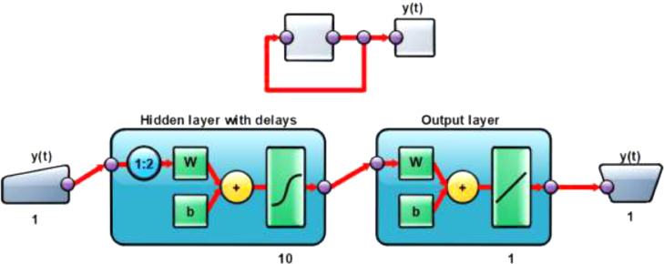
Unknown f function was modeled by using artificial neural network. Fig. 1 shows the NARNN 2-delay model consisting of 10 neurons. This neural network estimates the future value by looking at two historical data.
Fig. 1.
Main structure of NAR neural network model.
In order to determine the performance of the model, the values estimated by the neural network are compared with the results previously known and the difference is looked at. For high performance, it is desired that the difference value should be close to 0.
2.4. LSTM model
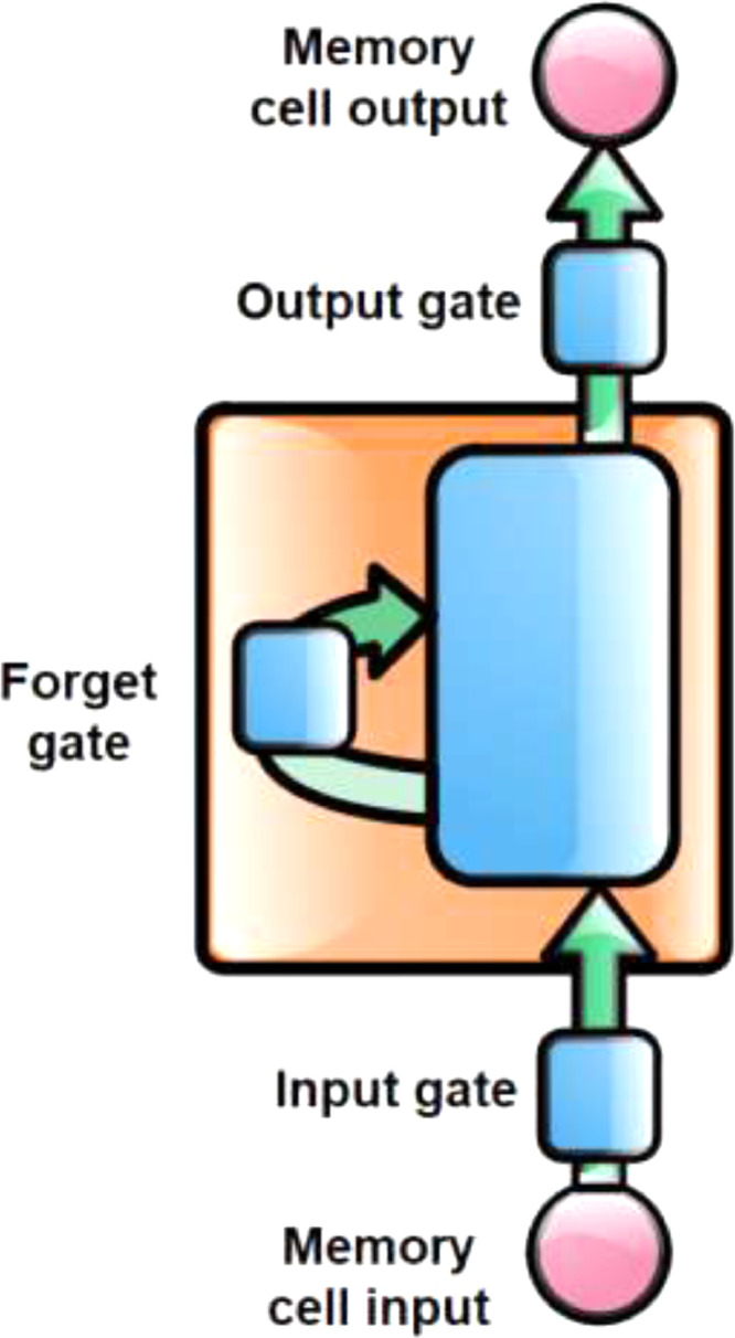
Long-short term memory (LSTM) is a machine learning algorithm with recurrent neural network architecture [14]. As a model, it stores the information learned in the short period and uses it for training in the long period. Therefore, long short-term memory contains units called "memory blocks" in hidden layer. These memory blocks can be defined as hidden units in traditional repeating neural networks. It contains one or more memory cells in the memory blocks. Each memory block contains input and output ports to control the flow of information. While the input gate controls the flow of input activation information in the memory cell, the output doors control the flow of output activation information. Later, a “forget gate” was added to the memory blocks. The forgetting gate scales the internal state of the cell, resets the memory of the cell, before the input activation through the cell's repetitive connection [15].
In order for the LSTM model to be better understood, the steps of the model must be examined. If the model input of the LSTM model is named xt at time t and the model output is ht, then the network to be created must first reset the output from the previous model at t.
| (8) |
The model should then be decided what information should be stored in the model. This process consists of two parts. First, the input gate layer decides which values to update. Then the sigmoid layer creates a vector containing possible new values. At the end of these processes, these two steps are combined and the input is updated.
| (9) |
| (10) |
| (11) |
Finally, the output of the network is decided. The result to be output here is formed from the decided part of the sigmoid gate.
| (12) |
| (13) |
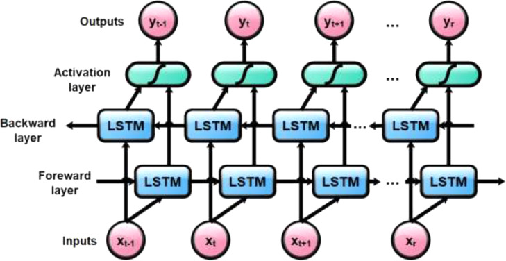
In the expressions below, tanh is utilized to scale the values into range – 1 to 1, W denotes the corresponding weight matrices, σ is the activation function which is taken as sigmoid, ft is forget function, Ct is candidate vector and ot is sigmoid function output. The output generated in the model is filtered output based on the model cell state. The internal architecture and LSTM architecture of the LSTM block used in this study are shown in Figs. 2 and 3 , respectively.
Fig. 2.
Internal architecture of LSTM.
Fig. 3.
LSTM architecture [11].
2.5. Model selection
The starting dates of the cases of the countries used in the study differ. At the same time, the number of days with the first 100 cases varies from country to country. This situation makes it difficult to make estimations by using the same model of 8 different countries. It is thought that health policies differing between countries, the level of interaction of people with non-patients, hygiene measures taken, and the total number of patients are important factors. However, in the study, all these factors were ignored and the problem was approached as a time series prediction problem.
The accuracy of a model can be evaluated by comparing the observed parameters and the estimated paremeters. In this work, six performance factor were analyzed for fair comparison. Mean Squared Error (MSE), Peak Signal-to-Noise Ratio (PSNR), Root-Mean-Square Error (RMSE), Normalized Root-Mean-Square Error (NRMSE), Mean Absolute Percentage Error (MAPE) and Symmetric Mean Absolute Percentage Error (SMAPE) can be calculated by using Eqs. (5–10), respectively [16].
| (5a) |
| (6a) |
| (7a) |
| (8a) |
| (9a) |
| (10a) |
In the above equations, RMSD is root-mean-square deviation, MAXf is peak value and SSE is error sum of squares.
3. Results and discussion
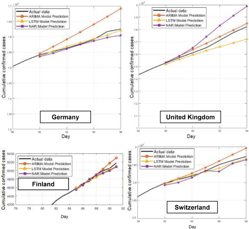
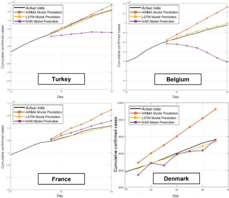
In this study, unlike other studies on COVID-19, data from different countries were estimated by three different methods. Fig. 4 shows 7-step estimates for Germany, United Kingdom, Finland and Switzerland. In Fig. 5 , the predictions of Turkey, Belgium, France and Denmark are illustrated. performance factors of the developed models are given in Table 2 .
Fig. 4.
Actual and predicted cumulative confirmed cases for Germany, United Kingdom, Finland and Switzerland.
Fig. 5.
Actual and predicted cumulative confirmed cases for Turkey, Belgium, France and Denmark.
Table 2.
Performance parameters of the models.
| Country | Model | Performance factor |
||||||
| MSE | PSNR | R value | RMSE | NRMSE | MAPE | SMAPE | ||
| Belgium | ARIMA | 5125899.8654 | -18.9668 | 0.997764295 | 2264.0450 | 0.6692 | 4.0080 | 3.9039 |
| NARNN | 19586992.1341 | -24.7888 | 0.991456949 | 4425.7193 | 1.3082 | 7.5148 | 7.9505 | |
| LSTM | 75089.6378 | -0.6249 | 0.999967249 | 274.0248 | 0.0810 | 0.5422 | 0.5407 | |
| Denmark | ARIMA | 323901.3369 | -6.9733 | 0.996006328 | 569.1233 | 0.6840 | 5.6512 | 5.4674 |
| NARNN | 21088.1719 | 4.8904 | 0.999739985 | 145.2176 | 0.1745 | 1.2583 | 1.2716 | |
| LSTM | 2974.5951 | 13.3965 | 0.999963324 | 54.5398 | 0.0655 | 0.5033 | 0.5051 | |
| Finland | ARIMA | 5046.1573 | 11.1011 | 0.999788236 | 71.0363 | 0.1178 | 1.1225 | 1.1140 |
| NARNN | 2846.3644 | 13.5878 | 0.999880551 | 53.3513 | 0.0884 | 0.9866 | 0.9904 | |
| LSTM | 2449.9178 | 14.2392 | 0.999897188 | 49.4966 | 0.0820 | 0.8492 | 0.8535 | |
| France | ARIMA | 15111600.3421 | -23.6623 | 0.999078692 | 3887.3641 | 0.6070 | 2.7102 | 2.6661 |
| NARNN | 1778423.6984 | -14.3695 | 0.999891575 | 1333.5755 | 0.2082 | 0.9834 | 0.9781 | |
| LSTM | 207675.3922 | -5.0430 | 0.999987339 | 455.7141 | 0.0711 | 0.3155 | 0.3159 | |
| Germany | ARIMA | 16826047.8234 | -24.1290 | 0.999327029 | 4101.9565 | 0.4929 | 2.2524 | 2.2202 |
| NARNN | 1252766.8129 | -12.8478 | 0.999949895 | 1119.2706 | 0.1345 | 0.5351 | 0.5375 | |
| LSTM | 324306.4567 | -6.9787 | 0.999987029 | 569.4791 | 0.0684 | 0.3083 | 0.3086 | |
| Switzerland | ARIMA | 15496.8206 | 6.2283 | 0.999982007 | 124.4862 | 0.1646 | 0.3422 | 0.3413 |
| NARNN | 9323.09771 | 8.4352 | 0.999989175 | 96.5561 | 0.1277 | 0.2730 | 0.2735 | |
| LSTM | 3121.2991 | 13.1874 | 0.999996376 | 55.8685 | 0.0739 | 0.1640 | 0.1641 | |
| Turkey | ARIMA | 2024356.6187 | -14.9320 | 0.999858804 | 1422.7988 | 0.1032 | 0.9209 | 0.9144 |
| NARNN | 69716342.4234 | -30.3025 | 0.995137376 | 8349.6312 | 0.6057 | 6.0581 | 6.2975 | |
| LSTM | 409936.1685 | -7.9963 | 0.999971407 | 640.26257 | 0.0464 | 0.4823 | 0.4835 | |
| United Kingdom | ARIMA | 5784979.5212 | -19.4922 | 0.999792714 | 2405.1984 | 0.0817 | 1.3075 | 1.2975 |
| NARNN | 99828262.3425 | -31.8617 | 0.996422984 | 9991.4094 | 0.3396 | 4.6611 | 4.5057 | |
| LSTM | 30054913.7467 | -26.6483 | 0.998923082 | 5482.2361 | 0.1863 | 2.5025 | 2.5512 | |
As can be seen from Fig. 4, it can be said that LSTM is a great success in predictions of Germany, Finland and Switzerland, while ARIMA is more successful in predictions of the United Kingdom. However, when looking at the MAPE values that can be seen from Table 2, it is seen that the performance rates for the United Kingdom are very close for LSTM and ARIMA. When looking at the countries in Fig. 5, it can be clearly seen that LSTM makes the most successful predictions. It can be seen that the country where LSTM makes the most successful estimation is Switzerland (MAPE = 0.1640) and the country that makes the most unsuccessful estimation is United Kingdom (MAPE = 2.5025). As to ARIMA and NARNN models, the best estimates made for Switzerland.
When all 7-step prediction graphs are examined, it is seen that LSTM model is clearly more successful than ARIMA and NAR models and it is the model that best matches the real data in the estimations made for all countries. While the ARIMA model makes more pessimistic estimates than other models, in general, the NARNN model made optimistic predictions below the real numbers.
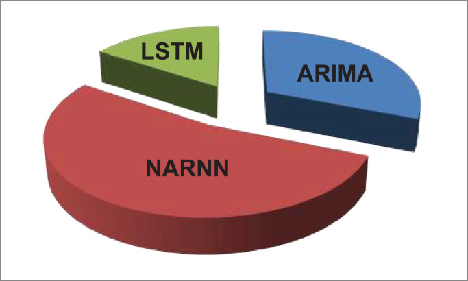
In this study, seven different model performance metrics were used to identify mathematical differences more clearly and fairly besides graphical comparisons (Table 1.). SMAPE values for LSTM, ARIMA and NARNN range from 0.16-2.55, 0.34-5.46 and 0.27-7.95, respectively. The smallest values for the metrics other than PSNR and R indicate the most successful model. The highest values in the PSNR metric and the values where the R value is closest to 1 indicate the most successful model. In addition, the weight of the total RMSE value by models is shown in Fig. 6 . Nevertheless, it is clearly seen that the lowest RMSE value is found for LSTM. Accordingly, it is clearly seen that the LSTM model is the most successful model for all country data examined within the scope of the study.
Fig. 6.
Distribution of total RMSE.
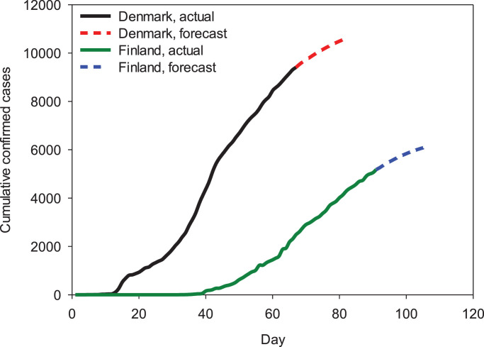
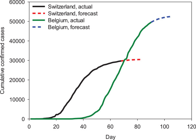
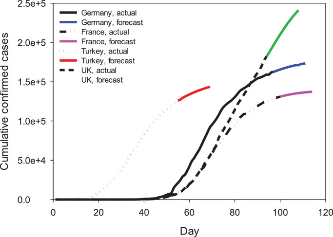
In the second stage of the study, the most successful model (LSTM) was provided to make predictions in a 14-day perspective that is yet to be known, and each prediction is presented in the form of graphs (Fig. 7, Fig. 8, Fig. 9 ). The reason for presenting three different graphs is that, countries that reach similar cumulative values can be understood in a more detailed way. When the future predictions of the model are analyzed, it is estimated that the UK's cumulative case data will maintain its upward trend, while the rate of increase will decrease for other countries.
Fig. 7.
Actual and forecasting cumulative confirmed cases for Denmark and Finland.
Fig. 8.
Actual and forecasting cumulative confirmed cases for Switzerland and Belgium.
Fig. 9.
Actual and forecasting cumulative confirmed cases for Germany, France, UK and Turkey.
For Denmark and Finland, 2-week predictions are expected to increase the cumulative confirmed cases data from 9407 to 10550 and 5179 to 6081, respectively. It has been determined that these values will increase from 29734 to 30482 and from 49517 to 52458, respectively, for Switzerland and Belgium. After 14 days of forecasting, the total cases in Germany, France, UK and Turkey were estimated to be 173378, 137260, 240879 and 143503. Optimistic progress is expected in all countries except the UK. Among the countries studied, the lowest number of cases was observed in Finland during the epidemic, while the highest rate of increase was observed in the UK. It is observed that the model achievements will increase when the number of days in which the outbreak data is diversified and the data collected is increased.
4. Conclusion and suggestions
The limited data on COVID-19 is quite challenging for modeling and prediction. In this study, the data from cumulative confirmed cases in some European countries are modeled using three different approaches. According to the results, it was determined that LSTM approach has much higher success compared to ARIMA and NARNN.
Later on, forward estimations were made with LSTM with high performance. Among the countries studied, the lowest number of cases was observed in Finland during the epidemic, while the highest rate of increase was observed in the UK. According to the 2-week prospective estimation study, in many countries, the total case increase rate is expected to decrease slightly. The study is carried out entirely by considering statistical data and methodologies, the effects of measures taken during the epidemic, compliance with hygiene rules or lockdown are ignored. Nevertheless, the rate of conformity of the developed prediction model with real data is very satisfactory and offers a strong projection for the near future. However, it is too early to draw a definitive conclusion due to the differences in available data, human behavior and measures taken on a country basis. It is observed that the model achievements will increase when the number of days in which the outbreak data is diversified and the data collected is increased.
Declaration of Competing Interest
The authors declare that they have no known competing financial interests or personal relationships that could have appeared to influence the work reported in this paper.
References
- 1.Rismanbaf A. Potential treatments for COVID-19; a narrative literature review. Arch Acad Emerg Med. 2020;8(1):e29. [PMC free article] [PubMed] [Google Scholar]
- 2.Chakraborty T., Ghosh I. Real-time forecasts and risk assessment of novel coronavirus (COVID-19) cases: a data-driven analysis. Chaos Solitons Fractals. 2020 doi: 10.1016/j.chaos.2020.109850. [DOI] [PMC free article] [PubMed] [Google Scholar]
- 3.Liu Q., Liu X., Jiang B., Yang W. Forecasting incidence of hemorrhagic fever with renal syndrome in China using ARIMA model. BMC Infect Dis. 2011;11(1) doi: 10.1186/1471-2334-11-218. [DOI] [PMC free article] [PubMed] [Google Scholar]
- 4.Cao L., Liu H., Li J., Yin X., Duan Y., Wang J. Relationship of meteorological factors and human brucellosis in Hebei Province, China. Sci Total Environ. 2020;703 doi: 10.1016/j.scitotenv.2019.135491. [DOI] [PubMed] [Google Scholar]
- 5.He Z., Tao H. Epidemiology and ARIMA model of positive-rate of influenza viruses among children in Wuhan, China: a nine-year retrospective study. Int J Infect Dis. 2018;74:61–70. doi: 10.1016/j.ijid.2018.07.003. [DOI] [PubMed] [Google Scholar]
- 6.Ceylan Z. Estimation of COVID-19 prevalence in Italy, Spain, and France. Sci Total Environ. 2020 doi: 10.1016/j.scitotenv.2020.138817. [DOI] [PMC free article] [PubMed] [Google Scholar]
- 7.Wu W., Guo J., An S., Guan P., Ren Y., Xia L., Zhou B. Comparison of two hybrid models for forecasting the incidence of hemorrhagic fever with renal syndrome in Jiangsu Province, China. PLoS One. 2015;10(8) doi: 10.1371/journal.pone.0135492. [DOI] [PMC free article] [PubMed] [Google Scholar]
- 8.Zhou L., Yu L., Wang Y., Lu Z., Tian L., Tan L. A hybrid model for predicting the prevalence of schistosomiasis in humans of Qianjiang City, China. PLoS ONE. 2014;9(8) doi: 10.1371/journal.pone.0104875. [DOI] [PMC free article] [PubMed] [Google Scholar]
- 9.Yu L., Zhou L., Tan L., Jiang H., Wang Y., Wei S. Application of a new hybrid model with seasonal auto-regressive integrated moving average (ARIMA) and nonlinear auto-regressive neural network (NARNN) in forecasting incidence cases of HFMD in Shenzhen, China. PLoS ONE. 2014;9(6):e98241. doi: 10.1371/journal.pone.0098241. [DOI] [PMC free article] [PubMed] [Google Scholar]
- 10.U J., Lu P., Kim C., Ryu U., Pak K. A new LSTM based reversal point prediction method using upward/downward reversal point feature sets. Chaos Solitons Fractals. 2020;132 doi: 10.1016/j.chaos.2019.109559. [DOI] [Google Scholar]
- 11.Chimmula V.K.R., Zhang L. Time series forecasting of COVID-19 transmission in Canada using LSTM networks. Chaos Solitons Fractals. 2020;135 doi: 10.1016/j.chaos.2020.109864. [DOI] [PMC free article] [PubMed] [Google Scholar]
- 12.Tomar A., Gupta N. Prediction for the spread of COVID-19 in India and effectiveness of preventive measures. Sci Total Environ. 2020 doi: 10.1016/j.scitotenv.2020.138762. [DOI] [PMC free article] [PubMed] [Google Scholar]
- 13.European Centre for Disease Prevention and Control, Geographic distribution of COVID-19 cases worldwide, Retrieved fromhttps://www.ecdc.europa.eu/en/publications-data/download-todays-data-geographic-distribution-covid-19-cases-worldwide
- 14.Hochreiter S., Schmidhuber J. Long short-term memory. Neural Comput. 1997;9(8):1735–1780. doi: 10.1162/neco.1997.9.8.1735. [DOI] [PubMed] [Google Scholar]
- 15.Gers F.A., Schmidhuber J., Cumming F.A. Learning to forget: continual prediction with LSTM. Neural Comput. 2000;12:2451–2471. doi: 10.1162/089976600300015015. [DOI] [PubMed] [Google Scholar]
- 16.Kırbaş İ, Tuncer A.D., Şirin C., Usta H. Modeling and developing a smart interface for various drying methods of pomelo fruit (Citrus maxima) peel using machine learning approaches. Comput Electron Agric. 2019;165 [Google Scholar]


