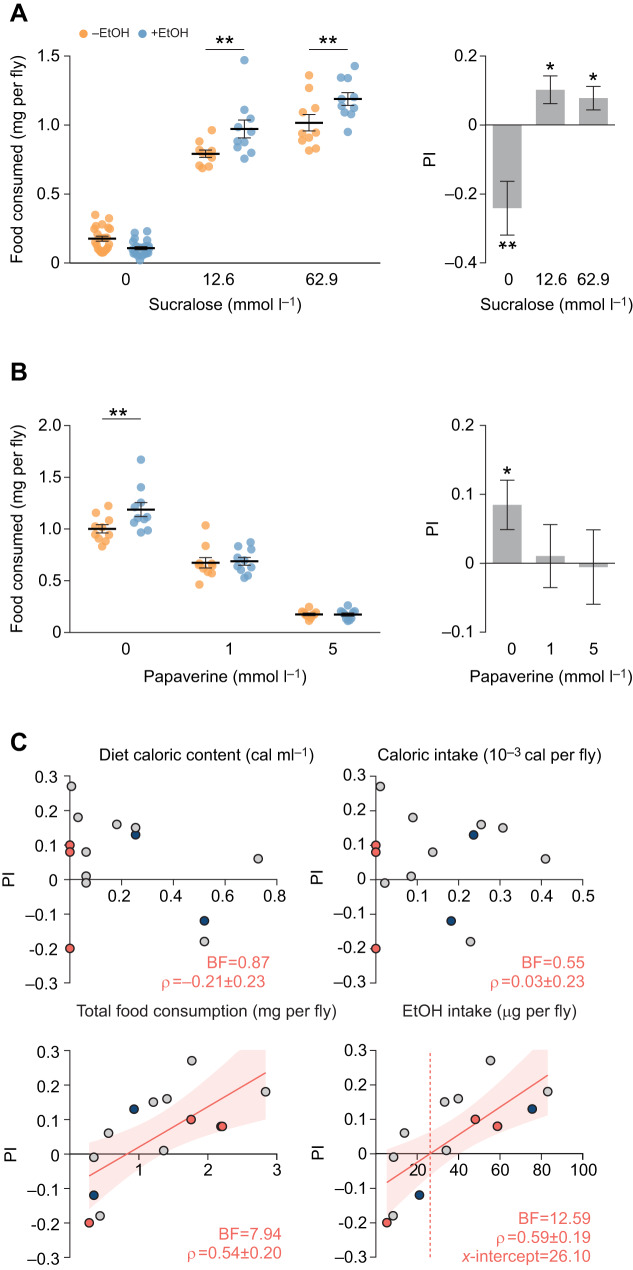
Fig. 2.

Absolute ethanol intake predicts ethanol preference. (A,B) Manipulating total food consumption with the non-nutritive tastants sucralose (sweet; A) or papaverine (bitter; supplied with 1.71% sucrose, equivalent to 50 mmol l⁻¹; B) alters ethanol preference. N=22 (0% sucralose) or 10 per diet. Significance: sucralose concentration, P<0.001; ethanol, P<0.01; sucralose×ethanol, P<0.001; papaverine concentration, P<0.001. Data shown are means±s.e.m. *P<0.05; **P<0.01; from two-way ANOVA followed by Tukey-adjusted post hoc comparison (raw consumption) or two-tailed one-sample Student's t-test (PI). (C) PI for ethanol mixed into various diets correlates with total food consumption and ethanol intake, but not with dietary caloric content. Each point represents PI on base diets of varying composition (N>10 per diet): gray, base diet with 5% ethanol; blue, base diet with 15% ethanol; red, non-caloric base diet with 5% ethanol. Results from Bayesian correlation analyses are summarized in each graph: BF, Bayesian factor; ρ, correlation estimate (median±median absolute deviation). Associations between PI and each of the parameters can be summarized as follows: dietary caloric content, anecdotal evidence for the absence of a negative association; caloric intake, anecdotal evidence for the absence of a positive association; total food consumption, moderate evidence for the existence of a positive association; ethanol intake, strong evidence for the existence of a positive association. Solid line and surrounding shaded area show linear regression and 95% confidence interval. Measurements reflect 24 h consumption in Canton-S males. For raw data and analysis, see Datasets 1 and 2.