Figure 2.

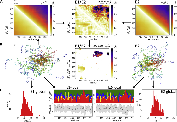
The ensemble-comparison approach: an overview. (A) Three heatmaps are displayed. Two represent a composite matrix for each of the ensembles E1 and E2 that are being compared. The upper triangle of each map displays the medians of the inter-residue distance distributions dμ(i,j). The lower triangle displays the SDs dσ(i,j) of the corresponding distributions. The third heatmap depicts the composite difference matrix (E1 and E2) between the two ensembles; its upper triangle depicts the Diff_dμ(i,j) matrix whose elements are the absolute differences between the dμ(i,j) distributions in the two ensembles; its lower triangles represents the absolute differences between the corresponding SDs of Diff_dσ(i,j) (see Materials and Methods for details). The inter-residue distances and differences thereof are given in angstroms. (B) A heatmap is given, highlighting only Sig_Diff_dμ(i,j) for the E1-E2 pair, i.e., elements of the Diff_dμ(i,j) matrix representing statistically significant differences between the corresponding d(i,j) distributions (p < 0.05) (upper triangle) and the corresponding Diff_dσ(i,j)-values (lower triangle). The highlighted differences concern d(i,j) distance distributions between a segment spanning residues 473–493 and the N-terminal region (residues 405–420) of the polypeptide. Flanking this map are cartoon models depicting the backbones of individual conformations of the E1 (left) and E2 (right) ensembles. The conformations are color coded from blue (N-terminus) to red (C-terminus) and are superimposed onto the equivalent helical segment (orange ribbon) in both ensembles. (C) Shown are the graphs of the local flexibility properties and conformational preferences of the E1-E2 ensembles (E1 local and E2 local). Shown are the lower graph plots of the medians and 95 percentile confidence interval of the local backbone RMSD distributions for conformations of the E1 and E2 ensembles. The upper graph shows the fraction of the conformations in each ensemble, adopting backbone (ϕ,ψ)-values mapped onto the corresponding four regions of the Ramachandran map (Fig. S10; red: α-helix; yellow: left-handed helix; blue: β-strand; and green: polyproline I and II) (17). The RMSD-values are computed as described in Materials and Methods. The local plots are flanked by bar graphs showing the Rg distributions of conformations in each ensemble (E1 global and E2 global) that indicate that the E2 ensemble is somewhat more compact than E1.