Figure 4.

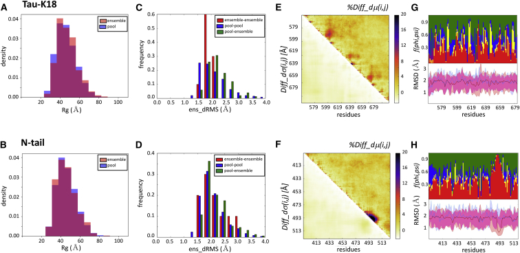
Experimental ensembles compared with their random-pool versions. The conformations of all five tau-K18 and MeV N-tail ensembles were combined and compared with those of the random-pool ensembles of each protein, respectively (25). (A and B) Shown are the histograms of the Rg distributions of the experimentally restrained versus the random-pool ensembles for the tau-K18 and MeV N-tail IDR domains, respectively. The tau-K18 ensembles are somewhat more compact than their random-pool version (p = 0.008), whereas both types of ensembles are indistinguishable for the MeV N-tail (p = 0.36). (C and D) Shown are the histograms of the pairwise ens_dRMS (in Angstroms)-values for the conformations of the experimentally restrained tau-K18 and MeV N-tail ensembles (red bars), random-pool versions of the corresponding proteins (blue bars), and pairs comprising members of both types of ensembles (green bars), respectively. (E and F) Shown are the heatmaps of the statistically significant portions of the normalized version of the difference matrix and the corresponding SD differences for the tau-K18 and MeV N-tail IDR domains versus their random-pool versions, respectively. The normalized version of the difference matrix %Diff_dμ(i,j) is defined as the percent difference between the dμ(i,j)-values from the two types of ensembles (see Materials and Methods). (G and H) Shown are twin graphs highlighting the regions of the IDRs with different backbone flexibility and local-structure preferences in conformations of the experimental and random-pool ensembles. Bottom graph: given are the medians and 95% confidence interval of the local backbone RMSD distributions for conformations of the merged pool (blue) and experimental (pink) ensembles of the tau-K18 (G) and MeV N-tail (H) ensembles, respectively, with the overlapping portions of the plots appearing in purple. Top graph: fractions of the conformations are given with specific (ϕ,ψ) preferences (see the legend of Fig. S10 for details).