FIG. 9.

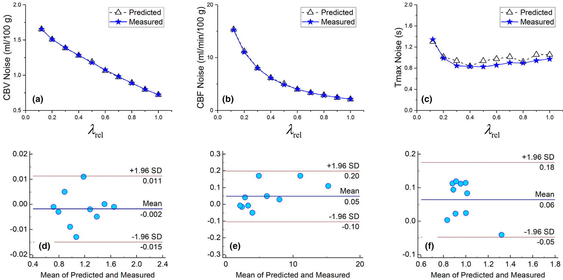
Comparison of measured and theoretically calculated σ_cbv* (a), σ_cbf* (b), and ${\sigma }_{t_{\text{max}}^{*}}$ (c) for gray matter in the digital phantom. The corresponding Bland–Altman plots are shown in (d), (e), and (f), respectively in the second row.