Fitting Penalized Logistic Regression Models Using QR Factorization

Abstract

The paper presents improvement of a commonly used learning algorithm for logistic regression. In the direct approach Newton method needs inversion of Hessian, what is cubic with respect to the number of attributes. We study a special case when the number of samples m is smaller than the number of attributes n, and we prove that using previously computed QR factorization of the data matrix, Hessian inversion in each step can be performed significantly faster, that is or instead of in the ordinary Newton optimization case. We show formally that it can be adopted very effectively to  penalized logistic regression and also, not so effectively but still competitively, for certain types of sparse penalty terms. This approach can be especially interesting for a large number of attributes and relatively small number of samples, what takes place in the so-called extreme learning. We present a comparison of our approach with commonly used learning tools.

Introduction

We consider a task of binary classification problem with n inputs and with one output. Let be a dense data matrix including m data samples and n attributes, and , are corresponding targets. We consider the case . In the following part bold capital letters denote matrices, bold lower case letters stand for vectors, and normal lower case for scalars. The paper concerns classification, but it is clear that the presented approach can be easily adopted to the linear regression model.

We consider a common logistic regression model in the following form:

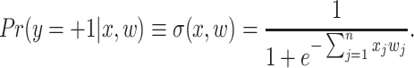1

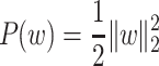
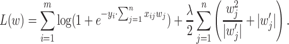
Learning of this model is typically reduced to the optimization of negative log-likelihood function (with added regularization in order to improve generalization and numerical stability):

2

where is a regularization parameter. Here we consider two separate cases:

1. rotationally invariant case, i.e. ,

2. other (possibly non-convex) cases, including .

Most common approaches include IRLS algorithm [7, 15] and direct Newton iterations [14]. Both approaches are very similar — here we consider Newton iterations:

3

where step size is chosen via backtracking line search [1]. Gradient and Hessian of have a form:

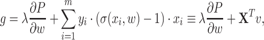4

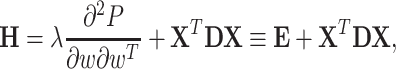5

where is a diagonal matrix, whose i-th entry equals , and .

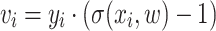Hessian is a sum of the matrix (second derivative of the penalty function multiplied by ) and the matrix . Depending on the penalty function P, the matrix may be: 1) scalar diagonal (), 2) non-scalar diagonal, 3) other type than diagonal. In this paper we investigate only cases 1) and 2).

Related Works. There are many approaches to learning logistic regression model, among them there are direct second order procedures like IRLS, Newton (with Hessian inversion using linear conjugate gradient) and first order procedures with nonlinear conjugate gradient as the most representative example. A short review can be found in [14]. The other group of methods includes second order procedures with Hessian approximation like L-BFGS [21] or fixed Hessian, or truncated Newton [2, 13]. Some of those techniques are implemented in scikit-learn [17], which is the main environment for our experiments. QR factorization is a common technique of fitting the linear regression model [9, 15].

Procedure of Optimization with QR Decomposition

Here we consider two cases. The number of samples and attributes leads to different kinds of factorization:

• LQ factorization for ,

• QR factorization for .

Since we assume , we consider LQ factorization of matrix :

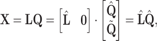6

where is lower triangular matrix, is orthogonal matrix and is semi-orthogonal matrix (, ). The result is essentially the same as if QR factorization of the matrix was performed.

Finding the Newton direction from the Eq. (3):

7

involves matrix inversion, which has complexity . A direct inversion of Hessian can be replaced (and improved) with a solution of the system of linear equations:

8

with the use of the conjugate gradient method. This Newton method with Hessian inversion using linear conjugate gradient is an initial point of our research. We show further how this approach can be improved using QR decomposition.

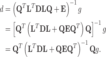
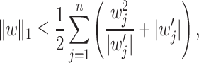
The Penalty Case and Rotational Invariance

In the -regularized case solution has a form:

9

Substituting for and for :

10

in the Eq. (9) leads to:

11

First, multiplication by transforms to the smaller space, then inversion is done in that space and finally, multiplication by brings solution back to the original space. However, all computation may be done in the smaller space (using instead of in the Eq. (9)) and only final solution is brought back to the original space — this approach is summarized in the Algorithm 1. In the experimental part this approach is called L2-QR.

This approach is not new [8, 16], however the use of this trick does not seem to be common in machine learning tools.

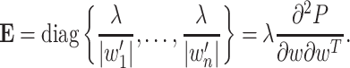
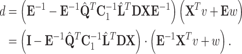
Rotational Variance

In the case of penalty functions whose Hessian is a non-scalar diagonal matrix, it is still possible to construct algorithm, which solves smaller problem via QR factorization.

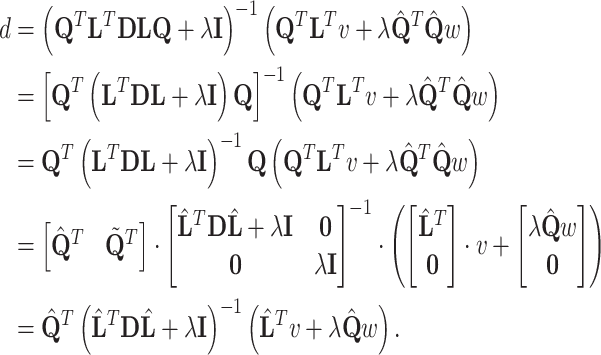
Consider again (5), (6) and (7):

12

Let 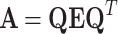, , so . Using Shermann-Morrison-Woodbury formula [5] we may write:

13

Let . Exploiting the structure of the matrices and (6) yields:

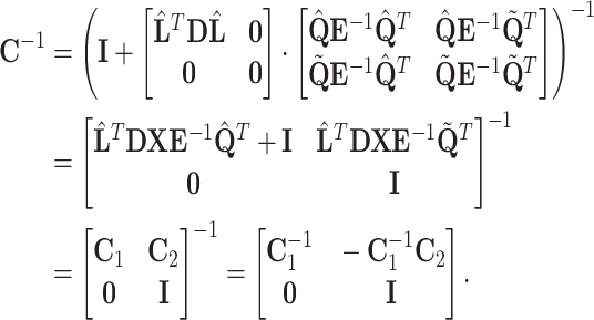14

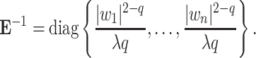
Hence only matrix of the size needs to be inverted — inversion of the diagonal matrix is trivial. Putting (14) and (13) into (12) and simplifying obtained expression results in:

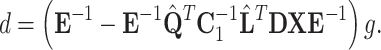15

This approach is summarized in the Algorithm 2.

Application to the Smooth Approximation. Every convex twice continuously differentiable regularizer can be put in place of ridge penalty and above procedure may be used to optimize such a problem. In this article we focused on the smoothly approximated -norm [12] via integral of hyperbolic tangent function:

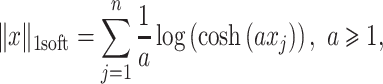16

and we call this model L1-QR-soft. In this case

Application to the Strict Penalty. Fan and Li proposed a unified algorithm for the minimization problem (2) via local quadratic approximations [3]. Here we use the idea presented by Krishnapuram [11], in which the following inequality is used:

17

what is true for any and equality holds if and only if .

Cost function has a form:

18

If we differentiate penalty term, we get:

19

where

Initial must be non zero (we set it to ), otherwise there is no progress. If falls below machine precision, we set it to zero.

Applying the idea of the QR factorization leads to the following result:

20

One can note that when is sparse, corresponding diagonal elements are 0. To avoid unneccessary multiplications by zero, we rewrite product as a sum of outer products:

21

where and are j-th columns of matrices and respectively. Similar concept is used when multiplying matrix by a vector e.g. : j-th element of the result equals . We refer to this model as L1-QR.

After obtaining direction we use backtracking line search1 with sufficient decrease condition given by Tseng and Yun [19] with one exception: if a unit step is already decent, we seek for a bigger step to ensure faster convergence.

Application to the Penalty. The idea described above can be directly applied to the “norms” [10] and we call it Lq-QR. Cost function has a form:

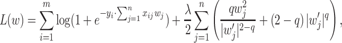22

where

Complexity of Proposed Methods

Cost of each iteration in the ordinary Newton method for logistic regression equals 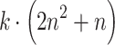, where k is the number of conjugate gradient iterations. In general , so in the worst case its complexity is .

Rotationally Invariant Case. QR factorization is done once and its complexity is . Using data transformed to the smaller space, each step of the Newton procedure is much cheaper and it requires about operations (cost of solving system of linear equations using conjugate gradient, ), what is in general.

As it is shown in the experimental part, this approach dominates other optimization methods (especially exact second order procedures). Looking at the above estimations, it is clear that the presented approach is especially attractive when .

Rotationally Variant Case. In the second case the most dominating operation comes from computation of the matrix in the Eq. (15). Due to dimensionality of matrices: and , the complexity of computation is — cost of inversion of the matrix is less important i.e. . In the case of penalty taking sparsity of into account reduces this complexity to , where is the number of non-zero coefficients.

Therefore theoretical upper bound on iteration for logistic regression with rotationally variant penalty function is , what is better than direct Newton approach. However, looking at (15), we see that the number of multiplications is large, thus a constant factor in this estimation is large.

Experimental Results

In the experimental part we present two cases: 1) learning ordinary logistic regression model, and 2) learning a 2-layer neural network via extreme learning paradigm. We use following datasets:

1. Artificial dataset with 100 informative attributes and 1000 redundant attributes, informative part was produced by function make_classification from package scikit-learn and whole set was transformed introducing correlations.

2. Two micro-array datasets: leukemia [6], prostate cancer [18].

3. Artificial non-linearly separable datasets: chessboard and , and two spirals — used for learning neural network.

As a reference we use solvers that are available in the package scikit-learn for LogisticRegression model i.e. for penalty we use: LibLinear [4] in two variants (primal and dual), L-BFGS, L2-NEWTON-CG; For sparse penalty functions we compare our solutions with two solvers available in the scikit-learn: LibLinear and SAGA.

For the case penalty we provide algorithm L2-QR presented in the Sect. 2.1. In the “sparse” case we compare three algorithms presented in the Sect. 2.2: L1-QR-soft, L1-QR and Lq-QR. Our approach L2-QR (Algorithm 1) is computationally equivalent to the L2-NEWTON-CG meaning that we solve an identical optimization problem (though in the smaller space). In the case of penalty all models should converge theoretically to the same solution, so differences in the final value of the objective function are caused by numerical issues (like numerical errors, approximations or exceeding the number of iterations without convergence). These differences affect the predictions on a test set.

The case of penalty is more complicated to compare. The L1-QR Algorithm is equivalent to the L1-Liblinear i.e. it minimizes the same cost function. Algorithm L1-QR-soft uses approximated -norm, and algorithm Lq-QR uses a bit different non-convex cost function which gives similar results to penalized regression for . We also should emphasize that SAGA algorithm does not optimize directly penalized log-likelihood function on the training set, but it is stochastic optimizer and it gives sometimes qualitatively different models. In the case L1-QR-soft final solution is sparse only approximately (and depends on a (16)), whereas other models produce strictly sparse models. The measure of sparsity is the number of non-zero coefficients. For L1-QR-soft we check the sparsity with a tolerance of order .

All algorithms were started with the same parameters: maximum number of iterations (1000) and tolerance (), and used the same learning and testing datasets. All algorithms depend on the regularization parameter C (or ). This parameter is selected in the cross-validation procedure from the same range. During experiments with artificial data we change the size of training subset. Experiments were performed on Intel Xeoen E5-2699v4 machine, in the one threaded envirovement (with parameters n_jobs=1 and MKL_NUM_THREADS=1).

Learning Ordinary Logistic Regression Model. In the first experiment, presented in the Fig. 1, we use an artificial highly correlated dataset (1). We used training/testing procedure for each size of learning data, and for each classifier we select optimal value of parameter using cross-validation. The number of samples varies from 20 to 300. As we can see, in the case penalty our solution using QR decomposition L2-QR gives better times of fitting than ordinary solvers available in the scikit-learn and all algorithms work nearly the same, only L2-lbfgs gives slightly different results. In the case of sparse penalty our algorithm L1-QR works faster than L1-Liblinear and obtains comparable but not identical results. For sparse case L1-SAGA gives best predictions (about 1–2% better than other sparse algorithms), but it produces the most dense solutions similarly like L1-QR-soft.

Fig. 1.

Comparison of algorithms for learning (a) and sparse (b) penalized logistic regressions on the artificial () dataset. Plots present time of cross-validation procedure (CV time), AUC on test set (auc test), and number of non-zero coefficients for sparse models (nnz coefs).

In the second experiment we used micro-array data with an original train and test sets. For those datasets quotients (samples/attributes) are fixed (about 0.005–0.01). The results are shown in Table 1 ( case) and in Table 2 ( case). Tables present mean values of times and cost functions, averaged over s. Whole traces over s are presented in the Fig. 2 and Fig. 3. For the case of penalty we notice that all tested algorithms give identical results looking at the quality of prediction and the cost function. However, time of fitting differs and the best algorithm is that, which uses QR factorization.

Table 1.

Experimental results for micro-array datasets and penalized logistic regressions. All solvers converge to the same solution, there are only differences in times.

Dataset	Classifier	[s]	Cost Fcn.
Golub	L2-Newton-CG	0.0520	1.17e+11	0.8571	0.8824
	L2-QR	0.0065	1.17e+11	0.8571	0.8824
	SAG	1.2560	1.17e+11	0.8571	0.8824
	Liblinear L2	0.0280	1.17e+11	0.8571	0.8824
	Liblinear L2 dual	0.0737	1.17e+11	0.8571	0.8824
	L-BFGS	0.0341	1.17e+11	0.8571	0.8824
Singh	L2-Newton-CG	0.6038	5.14e+11	0.9735	0.9706
	L2-QR	0.0418	5.14e+11	0.9735	0.9706
	SAG	5.2822	5.13e+11	0.9735	0.9706
	Liblinear L2	0.1991	5.14e+11	0.9735	0.9706
	Liblinear L2 dual	0.6083	5.14e+11	0.9735	0.9706
	L-BFGS	0.1192	5.14e+11	0.9735	0.9706

Table 2.

Experimental results for micro-array datasets and penalized logistic regressions. L1-QR solver converges to the same solution as L1-Liblinear, there are only difference in times. SAGA and L1-QR-soft gives different solution.

Dataset	Classifier	[s]	Cost Fcn.			NNZ coefs.
Golub	L1-QR-soft	8.121	2.74e+07	0.8929	0.9118	90.1
	-QR	0.544	2.80e+07	0.9393	0.95	9.1
	L1-QR	1.062	2.28e+07	0.8679	0.8912	10.2
	Liblinear	0.042	2.28e+07	0.8679	0.8912	10.4
	SAGA	4.532	2.78e+07	0.8857	0.9059	46.7
Singh	L1-QR-soft	51.042	6.74e+07	0.8753	0.8794	91.2
	-QR	3.941	8.65e+07	0.8893	0.9	13.4
	L1-QR	6.716	6.52e+07	0.8976	0.8912	20.1
	Liblinear	0.225	6.52e+07	0.8976	0.8912	20.2
	SAGA	21.251	7.11e+07	0.8869	0.8912	65.9

Fig. 2.

Comparison of algorithms learning penalized logistic regression on micro-array datasets for a sequence of s; mean values are presented in the Table 1.

Fig. 3.

Detailed comparison of algorithms learning penalized logistic regression on micro-array datasets for a sequence of s. Mean values for this case are presented in the Table 2.

For the case of sparse penalty functions only algorithms L1-Liblinear and L1-QR give quantitatively the same results, however L1-Liblinear works about ten times faster. Other models give qualitatively different results. Algorithm Lq-OR obtained the best sparsity and the best accuracy in prediction and was also slightly faster than L1-QR. Looking at the cost function with penalty we see that L1-Liblinear and L1-QR are the same, SAGA obtains worse cost function than even L1-QR-soft. We want to stress that scikit-learn provides only solvers for and penalty, not for general case .

Application to Extreme Learning and RVFL Networks. Random Vector Functional-link (RVFL) network is a method of learning two (or more) layer neural networks in two separate steps. In the first step coefficients for hidden neurons are chosen randomly and are fixed, and then in the second step learning algorithm is used only for the output layer. The second step is equivalent to learning the logistic regression model (a linear model with the sigmoid output function). Recently, this approach is also known as “extreme learning” (see: [20] for more references).

The output of neural network with a single hidden layer is given by:

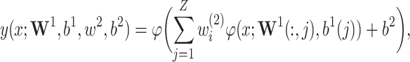23

where: Z is the number of hidden neurons, is the activation function.

In this experiment we choose randomly hidden layer coefficients and , with number of hidden neurons and next we learn the coefficients of the output layer: and using the new transformed data matrix:

For experiments we prepared the class ExtremeClassier (in scikit-learn paradigm) which depends on the number of hidden neurons Z, the kind of linear output classifier and its parameters. In the fitting part we ensure the same random part of classifier. In this experiment we also added a new model — multi-layer perceptron with two layers and with Z hidden neurons fitted in the standard way using L-BFGS algorithm (MLP-lbfgs).

Results of the experiment are presented in the Fig. 4. For each size of learning data and for each classifier we select optimal value of parameter using cross-validation. The number of samples varies from 20 to 300. As we can see, in both cases ( and sparse penalties) our solution using QR decomposition gives always better times of fitting than ordinary solvers available in the scikit-learn. Time of fitting of L1-QR is 2–5 times shorter than L1-Liblinear, especially for the case chessboard and two spirals. Looking at quality we see that sparse models are similar, but slightly different. For two spirals the best one is Lq-QR and it is also the sparsest model. Generally sparse models are better for two spirals and chessboard . The MLP model has the worst quality and comparable time of fitting to sparse regressions.

Fig. 4.

Experimental results for the extreme learning. Comparison on artificial datasets. CV time is the time of cross-validation procedure, fit time is the time of fitting for the best , auc test is the area under ROC on test dataset, and nnz coefs5 is the number of non-zero coefficients.

The experiment shows that use of QR factorization can effectively implement learning of RVFL network with different regularization terms. Moreover, we confirm that such learning works more stable than ordinary neural network learning algorithms, especially for the large number of hidden neurons. Exemplary decision boundaries, sparsity and found hidden neurons are shown in the Fig. 5.

Fig. 5.

Exemplary decision boundaries for different penalty functions (, with a smooth approximation of the absolute value function, , ) on used datasets. In the figure there are coefficients of the first layer of the neural network represented as lines — intensity and color represents magnitude and sign of the particular coefficient. (Color figure online)

Conclusion

In this paper we presented application of the QR matrix factorization to improve the Newton procedure for learning logistic regression models with different kind of penalties. We presented two approaches: rotationally invariant case with penalty, and general convex rotationally variant case with sparse penalty functions. Generally speaking, there is a strong evidence that use of QR factorization in the rotational invariant case can improve classical Newton-CG algorithm when . The most expensive operation in this approach is QR factorization itself, which is performed once at the beginning. Our experiments showed also that this approach, for surpasses also other algorithms approximating Hessian like L-BFGS and truncated Newton method (used in Liblinear). In this case we have shown that theoretical upper bound on cost of Newton iteration is .

We showed also that using QR decomposition and Shermann-Morrison-Woodbury formula we can solve a problem of learning the regression model with different sparse penalty functions. Actually, improvement in this case is not as strong as in the case of penalty, however we proved that using QR factorization we obtain theoretical upper bound significantly better than for general Newton-CG procedure. In fact, the Newton iterations in this case have the same cost as the initial cost of the QR decomposition i.e. . Numerical experiments revealed that for more difficult and correlated data (e.g. for extreme learning) such approach may work faster than L1-Liblinear. However, we should admit that in a typical and simpler cases L1-Liblinear may be faster.

References

- 1.Boyd S, Vandenberghe L. Convex Optimization. New York: Cambridge University Press; 2004. [Google Scholar]
- 2.Dai YH. On the nonmonotone line search. J. Optim. Theory Appl. 2002;112(2):315–330. doi: 10.1023/A:1013653923062. [DOI] [Google Scholar]
- 3.Fan J, Li R. Variable selection via nonconcave penalized likelihood and its oracle properties. J. Am. Stat. Assoc. 2001;96(456):1348–1360. doi: 10.1198/016214501753382273. [DOI] [Google Scholar]
- 4.Fan RE, Chang KW, Hsieh CJ, Wang XR, Lin CJ. LIBLINEAR: a library for large linear classification. J. Mach. Learn. Res. 2008;9:1871–1874. [Google Scholar]
- 5.Golub, G., Van Loan, C.: Matrix Computations. Johns Hopkins Studies in the Mathematical Sciences, Johns Hopkins University Press (2013)
- 6.Golub TR, et al. Molecular classification of cancer: class discovery and class prediction by gene expression monitoring. Science. 1999;286(5439):531–537. doi: 10.1126/science.286.5439.531. [DOI] [PubMed] [Google Scholar]
- 7.Green PJ. Iteratively reweighted least squares for maximum likelihood estimation, and some robust and resistant alternatives (with discussion) J. R. Stat. Soc. Ser. B Methodol. 1984;46:149–192. [Google Scholar]
-
8.Hastie, T., Tibshirani, R.: Expression arrays and the
problem (2003)
- 9.Hastie T, Tibshirani R, Friedman J. The Elements of Statistical Learning. New York: Springer; 2001. [Google Scholar]
10.Kabán A, Durrant RJ. Learning with
vs
vs  -norm regularisation with exponentially many irrelevant features. In: Daelemans W, Goethals B, Morik K, editors. Machine Learning and Knowledge Discovery in Databases. Heidelberg: Springer; 2008. pp. 580–596. [Google Scholar]
- 11.Krishnapuram B, Carin L, Figueiredo MAT, Hartemink A. Sparse multinomial logistic regression: fast algorithms and generalization bounds. IEEE Trans. Pattern Anal. Mach. Intell. 2005;27(6):957–968. doi: 10.1109/TPAMI.2005.127. [DOI] [PubMed] [Google Scholar]
- 12.Lee YJ, Mangasarian O. SSVM: a smooth support vector machine for classification. Comput. Optim. Appl. 2001;20:5–22. doi: 10.1023/A:1011215321374. [DOI] [Google Scholar]
- 13.Lin CJ, Weng RC, Keerthi SS. Trust region Newton method for logistic regression. J. Mach. Learn. Res. 2008;9:627–650. [Google Scholar]
- 14.Minka, T.P.: A comparison of numerical optimizers for logistic regression (2003). https://tminka.github.io/papers/logreg/minka-logreg.pdf
- 15.Murphy KP. Machine Learning: A Probabilistic Perspective. Cambridge: MIT Press; 2013. [Google Scholar]
16.Ng, A.Y.: Feature selection,
vs.
vs.  regularization, and rotational invariance. In: Proceedings of the Twenty-First International Conference on Machine Learning, ICML 2004, pp. 78–85. ACM, New York (2004)
- 17.Pedregosa F, et al. Scikit-learn: machine learning in python. J. Mach. Learn. Res. 2011;12:2825–2830. [Google Scholar]
- 18.Singh S, Skanda S, Scott S, Arie B, Sujata P, Gurmit S. Overexpression of vimentin: role in the invasive phenotype in an androgen-independent model of prostate cancer. Cancer Res. 2003;63(9):2306–2311. [PubMed] [Google Scholar]
- 19.Tseng P, Yun S. A coordinate gradient descent method for nonsmooth separable minimization. Math. Program. 2009;117:387–423. doi: 10.1007/s10107-007-0170-0. [DOI] [Google Scholar]
- 20.Wang LP, Wan CR. Comments on “the extreme learning machine”. IEEE Trans. Neural Netw. 2008;19(8):1494–1495. doi: 10.1109/TNN.2008.2002273. [DOI] [PubMed] [Google Scholar]
- 21.Zhu C, Byrd RH, Lu P, Nocedal J. Algorithm 778: L-BFGS-B: Fortran subroutines for large-scale bound-constrained optimization. ACM Trans. Math. Softw. 1997;23(4):550–560. doi: 10.1145/279232.279236. [DOI] [Google Scholar]