Improving Clinical Translation of Machine Learning Approaches Through Clinician-Tailored Visual Displays of Black Box Algorithms: Development and Validation

Abstract

Background

Despite the promise of machine learning (ML) to inform individualized medical care, the clinical utility of ML in medicine has been limited by the minimal interpretability and black box nature of these algorithms.

Objective

The study aimed to demonstrate a general and simple framework for generating clinically relevant and interpretable visualizations of black box predictions to aid in the clinical translation of ML.

Methods

To obtain improved transparency of ML, simplified models and visual displays can be generated using common methods from clinical practice such as decision trees and effect plots. We illustrated the approach based on postprocessing of ML predictions, in this case random forest predictions, and applied the method to data from the Left Ventricular (LV) Structural Predictors of Sudden Cardiac Death (SCD) Registry for individualized risk prediction of SCD, a leading cause of death.

Results

With the LV Structural Predictors of SCD Registry data, SCD risk predictions are obtained from a random forest algorithm that identifies the most important predictors, nonlinearities, and interactions among a large number of variables while naturally accounting for missing data. The black box predictions are postprocessed using classification and regression trees into a clinically relevant and interpretable visualization. The method also quantifies the relative importance of an individual or a combination of predictors. Several risk factors (heart failure hospitalization, cardiac magnetic resonance imaging indices, and serum concentration of systemic inflammation) can be clearly visualized as branch points of a decision tree to discriminate between low-, intermediate-, and high-risk patients.

Conclusions

Through a clinically important example, we illustrate a general and simple approach to increase the clinical translation of ML through clinician-tailored visual displays of results from black box algorithms. We illustrate this general model-agnostic framework by applying it to SCD risk prediction. Although we illustrate the methods using SCD prediction with random forest, the methods presented are applicable more broadly to improving the clinical translation of ML, regardless of the specific ML algorithm or clinical application. As any trained predictive model can be summarized in this manner to a prespecified level of precision, we encourage the use of simplified visual displays as an adjunct to the complex predictive model. Overall, this framework can allow clinicians to peek inside the black box and develop a deeper understanding of the most important features from a model to gain trust in the predictions and confidence in applying them to clinical care.

Introduction

Background

There is growing interest in benefiting from the predictive power of machine learning (ML) to improve the outcomes of medical care at more affordable costs. Although notable for their impressive predictive ability, ML black box predictions are often characterized by minimal interpretability, limiting their clinical adoption despite their promise for improving health care [1-6]. As a result, there is growing emphasis on the field of interpretable ML or explainable Artificial Intelligence to provide explanations of how models make their decisions [6-8]. However, the lack of understanding of how ML predictions are generated and the complex relationships between the predictors and outcomes are still obstacles to the adoption of ML in clinical practice.

Many approaches have been developed to explain predictions and determine ML feature importance and effect, but they have limited adoption in real-world clinical applications [9-12]. There have been previous proposals to stack ML methods or to use rule extraction with ML output to produce simpler summaries, but because of their inherent complexities or lack of clinical applications, these tools are seldom used in medicine [13-16].

Objectives

To accelerate the integration of ML into clinical care, an emphasis on the personalization of these tools for the end user is crucial. Our work is motivated by the well-known clinical challenge of measuring an individual's risk of sudden cardiac death (SCD), a leading cause of death with inherently complex pathophysiology that lends itself to novel approaches [17-22]. Although we focus here on SCD as an illustrative example, the methods we present are applicable more broadly to improving clinical translation of ML, regardless of the specific ML algorithm or clinical application. The contribution of this work is a general framework for translating complex black box predictions into easily understood representations through commonly encountered clinical summaries. Overall, we emphasize the need for multidisciplinary teams to create clinician-tailored visual displays that provide interpretability in ways that are personalized to the clinician’s preferences for understanding ML predictions to aid in effective clinical translation of ML.

Methods

Data Source

The Left Ventricular (LV) Structural Predictors of SCD Registry is a prospective observational registry (clinicaltrials.gov, NCT01076660), which enrolled 382 patients for the primary end point of an adjudicated appropriate implantable cardioverter defibrillator firing for ventricular tachycardia or ventricular fibrillation or SCD not aborted by the device [23-29]. In the 8-year follow-up, 75 individuals had the primary outcome.

Modeling

Our ML approach is based on the random forest (RF) algorithm implemented in the randomForestSRC R package [30] extended to time-varying SCD risk prediction [31]. RF is an ensemble learning method based on a collection of decision trees, where the overall RF prediction is the ensemble average or majority vote. Random sampling of predictor variables at each decision tree node and bootstrapping the original training data decrease the correlation among the trees in the forest to allow for impressive predictive performance [32,33]. For our RF, the predictors included demographics, comorbidities, medications, electrophysiologic parameters, laboratory values, LV ejection fraction by echocardiography, and cardiac magnetic resonance (CMR) imaging indices, summarized in Table 1.

Table 1.

Patient characteristics in the Left Ventricular Structural Predictors of Sudden Cardiac Death Registry (N=382).

Variables			No. of SCDa event (n=307)		Patient with SCD event (n=75)		P valueb
Demographics and clinical characteristics
	Age (years), mean (SD)			57 (13)		57 (12)		.75
	Male, n (%)			211 (68.7)		63 (84)		.01
	Race, n (%)							.66
		White	200 (65.1)		51 (68)
		African American	99 (32)		21 (28)
		Other	8 (3)		3 (4)
	Body surface area (m2), mean (SD)			1.98 (0.28)		2.05 (0.28)		.07
	Ischemic cardiomyopathy etiology, n (%)			149 (48.5)		44 (59)		.15
	Years from incident MIc or cardiomyopathy diagnosis, mean (SD)			3.83 (5.18)		5.43 (5.61)		.02
	NYHAd functional class, n (%)							.55
		I	64 (21)		20 (27)
		II	137 (44.6)		31 (41)
		III	106 (34.5)		24 (32)
	One or more heart failure hospitalizations, n (%)			0 (0)		19 (25.3)		<.001
Cardiac risk factors, n (%)
	Hypertension			180 (58.6)		44 (59)		>.99
	Hypercholesterolemia			180 (58.6)		45 (60)		.93
	Diabetes			85 (28)		19 (25)		.79
	Nicotine use			133 (43.3)		44 (59)		.02
Medication usage, n (%)
	ACEe-inhibitor or ARBf			275 (89.6)		66 (88)		.85
	Beta-blocker			288 (93.8)		68 (91)		.48
	Lipid-lowering			199 (64.8)		56 (75)		.14
	Antiarrhythmics (amiodarone)			18 (6)		8 (11)		.22
	Diuretics			173 (56.4)		54 (72)		.02
	Digoxin			50 (16)		16 (21)		.39
	Aldosterone inhibitor			80 (26)		21 (28)		.85
	Aspirin			215 (70.0)		55 (73)		.67
Electrophysiologic variables
	Prior atrial fibrillation, n (%)			51 (17)		14 (19)		.80
	Ventricular rate (bpm), mean (SD)			73 (14)		70 (14)		.06
	QRS duration (ms), mean (SD)			118 (31)		122 (27)		.30
	Presence of LBBBg, n (%)			79 (26)		14 (19)		.26
	Biventricular ICDh, n (%)			90 (29)		17 (23)		.31
Laboratory values or biomarkers
	Sodium (mEq/L), mean (SD)			139 (3)		139 (3)		.73
	Potassium (mEq/L), mean (SD)			4.26 (0.42)		4.27 (0.39)		.87
	Creatinine (mEq/L), mean (SD)			1.07 (0.59)		1.09 (0.33)		.81
	eGFRi (mL/min/1.73 m2), mean (SD)			81 (24)		80 (21)		.80
	Blood urea nitrogen (mg/dL), mean (SD)			19.62 (8.72)		20.28 (8.33)		.55
	Glucose (mg/dL), mean (SD)			120 (53)		113 (34)		.23
	Hematocrit (%), mean (SD)			40 (4)		41 (5)		.03
	hsCRPj (µg/mL), mean (SD)			6.89 (12.87)		9.10 (16.29)		.22
	NT-proBNPk (ng/L), mean (SD)			2704 (6736)		2519 (1902)		.82
	IL-6l (pg/mL), mean (SD)			3.05 (5.36)		4.32 (6.28)		.12
	IL-10m (pg/mL), mean (SD)			10.74 (49.67)		13.67 (59.94)		.70
	TNF-αRIIn (pg/mL), mean (SD)			3425 (1700)		3456 (1671)		.90
	cTnTo (ng/mL), mean (SD)			0.03 (0.08)		0.02 (0.05)		.62
	cTnIp (ng/mL), mean (SD)			0.10 (0.28)		0.10 (0.25)		.98
	CK-MBq (ng/mL), mean (SD)			3.94 (5.77)		3.87 (3.86)		.93
	Myoglobin (ng/mL), mean (SD)			31.37 (30.80)		37.13 (41.53)		.31
LVEFr: NonCMRs LVEF (%), mean (SD)			24.2 (7.6)		23.0 (7.4)		.19
CMR structural and functional indices
	LVEF (%), mean (SD)			27.8 (10.3)		25.1 (8.8)		.04
	LVt end-diastolic volume index (ml/m2), mean (SD)			122.3 (39.9)		136.2 (48.4)		.01
	LV end-systolic volume index (ml/m2), mean (SD)			91.5 (39.1)		104.3 (45.2)		.02
	LV mass index (ml/m2), mean (SD)			75.1 (24.4)		80.3 (21.2)		.09
CMR hyperenhancement
	LGEu present (%), mean (SD)			176 (66)		56 (86)		.002
	Gray zone (g), mean (SD)			8.8 (11.6)		13.8 (12.2)		.002
	Core (g), mean (SD)			12.4 (14.9)		17.7 (15.1)		.01
	Total scar (g), mean (SD)			21.1 (25.4)		31.3 (25.6)		.004

^aSCD: sudden cardiac death.

^bP values <.05 are italicized.

^cMI: myocardial infarction.

^dNYHA: New York Heart Association.

^eACE: angiotensin-converting enzyme.

^fARB: angiotensin II receptor blocker.

^gLBBB: left bundle branch block.

^hICD: implantable cardioverter defibrillator.

ⁱeGFR: estimated glomerular filtration rate.

^jhsCRP: high-sensitivity C-reactive protein.

^kNT-proBNP: N-terminal pro-b-type natriuretic peptide.

^lIL-6: interleukin-6.

^mIL-10: interleukin-10.

ⁿTNF-αRII: tumor necrosis factor alpha R II.

^ocTnT: cardiac troponin T.

^pcTnI: cardiac troponin I.

^qCK-MB: creatine kinase MB.

^rLVEF: left ventricular ejection fraction.

^sCMR: cardiac magnetic resonance.

^tLV: left ventricular.

^uLGE: late gadolinium enhancement.

Interpretability

To communicate the results from ML models, such as our RF for SCD predictions, we develop representative interpretable summaries. As illustrated in Figure 1, the following general steps can be employed to create simplified representations of any black box prediction:

Figure 1.

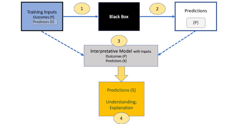
Steps to present machine learning (ML) predictions in an interpretable manner: The black box algorithm is applied to input data comprising outcomes (Y) and predictors (X) to obtain black-box predictions (P) of the input outcomes. The original X variables and the black-box predictions (P) are inputs to a simple model or algorithm, for example a single tree, whose predictions (S) are sufficiently close to (P) but more easily understood and explained.

1. Train the ML model with the input features (X) and the outcome of interest (Y).

2. Obtain the predicted values (P) from the ML model using cross-validation, a separate test dataset, or another data-division approach to ensure that predictions are not obtained from the same dataset used to train the model.

3. Train a simple, interpretable, and clinically understood model, such as a decision tree [34] or a linear or logistic regression model [35], using the predicted values (P) from the ML model as the outcome of interest and the corresponding input variables (X) from the original training dataset.

4. Obtain the predicted values (S) from the interpretive model. Calculate how close S is to P, that is how well the simplified model represents the ML model, using a measure such as R², defined as provided in Figure 2.

Figure 2.

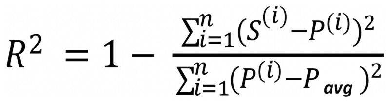
R² equation where i=1 to n observations evaluated. S⁽ⁱ⁾ denotes the prediction for the i^th observation using the simplified model, P⁽ⁱ⁾ denotes the prediction for the ith observation using the ML model, and P_avg denotes the average prediction from the ML model.

Note that the interpretative tree can be grown sufficiently large such that R² is arbitrarily close to 1. If a simple tree has a small R², extra caution should be exercised to avoid overinterpreting the simplified model. In contrast, if R² is high, the simplified model may be considered as an alternative to the actual ML model for obtaining future predictions in a simplified manner [36,37]. This model-agnostic approach to obtain a simplified summary of the ML model is shown in Figure 1.

By using a single tree as a summary of the RF predictions, we can quantify the importance of individual variables or groups of variables. A useful measure of the total effect on outcome Y of predictor (or group of predictors) X₁ is obtained by summing the improvements in prediction error (deviance) over all of the X₁ splits in the interpretative tree.

To present results in other ways familiar to clinicians, predictor effects can be communicated in plots where risk ratios are presented [38]. We created plots based on the relationship between the predictor variables and predicted risks. For categorical variables, risk ratios are calculated by comparing risks for different levels of the categorical variable (eg, risk ratio=[average predicted risk for males]/[average predicted risk for females] ). For continuous variables, risk ratios are calculated by comparing risks for different ranges of the continuous variable (eg, risk ratio=[average predicted risk for upper tertile of age]/[average predicted risk for lower tertile of age]). CIs for these risk ratios were generated through nonparametric bootstrap approaches [39]. All analyses were conducted using R 3.5.1 (R Foundation) [40].

Results

Global Summary Visualization

Using data from the LV Structural Predictors of SCD Registry, a global summary for SCD risk prediction is obtained by fitting a single decision tree to RF predictions using as inputs the same covariates used in the RF and the outcome as the RF predictions. Figure 3 shows a global summary tree of the RF model for SCD prediction. Several risk factors appear as early split nodes in the decision tree representing key variables that discriminate between low -, intermediate -, and high-risk patients, including heart failure (HF) hospitalization history, CMR imaging indices (ie, LV end-diastolic volume index, and total scar and gray zone mass), and a measure of systemic inflammation, interleukin-6 (IL-6).

Figure 3.

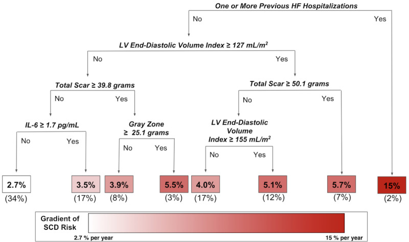
Global summary tree of random forest (RF) model for sudden cardiac death (SCD) prediction: Several risk factors (namely heart failure hospitalization, several cardiac magnetic resonance imaging indices, and interleukin-6 [IL-6], a marker of inflammation) discriminate between low-, intermediate-, and high- risk patients. Decision rules in the tree are shown in bold italics. The 1-year risks of SCD are shown in the boxes at the bottom of the decision tree. The boxes are colored according to the magnitude of the percent per year risk, with white corresponding to the lowest risk subgroup and dark red corresponding to the highest risk subgroup. Percentages in parentheses at the bottom of the boxes are the proportions of the total training data that belong to each of the risk subgroups. R² is 0.88 for how well this global summary tree represents the RF model. HF: heart failure; LV: left ventricular.

Risk Ratio and Variable Importance

Figure 4 shows the risk ratio plot for predictors identified as splitting variables in the global tree summary model for our RF SCD prediction example presented in Figure 3. The largest risk ratio is for HF hospitalization history before an arrhythmic event, indicating that individuals with 1 or more preceding HF hospitalizations are at 4.06 (95% CI 2.82-5.30) times higher risk of SCD than individuals without hospitalizations for HF. Comparing the risk for individuals in the upper versus lower tertile for CMR imaging variables and IL-6 demonstrates that higher values for these variables suggest a higher SCD risk. Specifically, the risk ratios were 1.54 (95% CI 1.14-1.93) for an LV end-diastolic volume index above 133 mL/m² versus below 102 mL/m²; 1.48 (95% CI 1.04-1.92) for a total scar mass above 30.79 g versus below 1.48 g; 1.48 (95% CI 1.04-1.91) for a gray zone mass above 11.37 g versus below 0.40 g, and 1.38 (95% CI 1.11-1.66) for IL-6 above 2.15 pg/mL versus below 1.04 pg/mL.

Figure 4.

Visualization of predictor effects in random forest (RF) model for sudden cardiac death (SCD) prediction: Risk ratio point estimates and the 95% confidence intervals generated from 500 bootstrap replications are shown for the RF model for SCD risk prediction. The largest risk ratio is between individuals who never experienced a heart failure hospitalization and those who experienced one or more heart failure hospitalizations. The other risk ratio comparisons show the risk ratios between individuals grouped into different categories based upon inflammation or cardiac magnetic resonance (CMR) imaging variables indicating the structural and functional properties of the heart. HF: heart failure; IL-6: interleukin 6; LV: left ventricular.

Table 2 lists the predictor variables in their order of importance in the single interpretative tree shown in Figure 3. Their ranking is based on the fraction of total variation (deviance) in the ML predictions they explain in 1 or more splits in the single tree shown in Figure 3. Although there are only 8 terminal nodes in the tree, the tree explains 88% of the information in the predictions from the black box RF. Additionally, trees inherently identify interactions. Note that after the first split on whether or not a person had a prior hospitalization for HF, the imaging variable only predicted risk among persons without prior hospitalization. This asymmetry indicates that the absence of a prior HF hospitalization strongly interacts with the cardiac imaging variables.

Table 2.

This table summarizes the global summary tree (shown in Figure 3) with an analysis of the variation (deviance) in the predicted values (P) from the machine learning (ML) model explained by the predictors in the global summary tree. The number of splits contributed by each variable in the global summary tree is enumerated along with the deviance and the percentage of the deviance explained. The predictors' ranked importance (ordered from most to least important from left to right in the table) is determined from the percentage of the deviance explained.

Split variable	HFa hospitalization history	LVb end-diastolic volume index	Total scar	Inflammation (IL-6c)	Gray zone	Tree total	MLd total
Number of splits	1	2	2	1	1	7	N/Ae
Deviance explained	1.26	0.255	0.100	0.034	0.020	1.67	1.89
Percentage of deviance explained	66.6	13.5	5.2	1.7	1.1	0.88f	100

^aHF: heart failure.

^bLV: left ventricular.

^cIL-6: interleukin 6.

^dML: machine learning.

^eN/A: not applicable.

^fThis corresponds to the R² value (0.88) obtained when using the equation shown in Figure 3 for the calculations.

Discussion

Principal Findings

We demonstrate that it is possible to obtain improved transparency of ML by generating simplified models and visual displays adapted from those used commonly in clinical practice. As a specific example of this framework, we use RF extended to survival analysis with time-varying covariates for individualized SCD risk prediction. Commonly used methods for SCD risk prediction, such as Cox proportional hazards regression, do not automatically account for nonlinear and interaction effects or facilitate the application to individualized risk prediction [41,42]. In contrast to traditional regression strategies or parametric approaches that make assumptions about the underlying model, ML, such as RF, employs nonparametric algorithms that allow the data to speak for themselves and perform as powerful methods for individualized predictions [32,43-45]. RFs, as ensembles of decision trees, are not easily interpretable even though single decision trees are popular in medicine because of their intuitiveness and comparability to how a clinician tends to think through a case. The framework introduced in this work provides a methodology to increase ML transparency through representative interpretable summaries.

Because this framework for interpretability is model-agnostic, the user may benefit from ML’s high predictive performance while also gaining insights into how predictions were generated. Despite the complexity of the original algorithm, these methods for interpretability only depend on the inputs upon which the black box was trained and the corresponding outputs from the black box, namely its predictions. Thus, any method for prediction can be explained to an extent in a simplified manner. In a situation where it is not possible to capture the variation in ML predictions with a simple summary, the proposed method signals this problem through a natural comparison of the similarity between the predicted values from the ML and its approximating interpretative model. This approach extends prior research in mimic learning and post hoc explanations of the black box predictions [46,47]. This paper emphasizes the clinician’s perspective as the end user experienced with tree-based reasoning as a natural correlate of clinical reasoning.

To implement ML in clinical practice, it is essential to provide user-centric tools that allow clinicians to gain understanding and trust in their predictions [48]. Developing visualizations that are easy to interpret and based upon familiar ways clinicians understand algorithms or results can help communicate ML predictions. For example, simplifying RFs into a single decision tree produces a visualization that reflects medical treatment or diagnostic decision making in clinical practice. Although we illustrate the simplified model with a decision tree, other models such as linear regression can also be presented. Additionally, providing visual displays of risk ratio estimates in a manner similar to those presented in the medical literature may help clinicians gain an understanding of ML predictions.

Developing interpretable predictions is particularly important in the application of ML to health care because of the unique challenges related to medical ethics and regulatory or legal considerations [48]. Explanations that describe predictions can facilitate trust, especially when the explanations are consistent with domain knowledge or extend upon what is currently known [48]. For instance, in our illustrative example of SCD prediction in the LV Structural Predictors of SCD Registry, the key risk factors are HF hospitalization history, CMR imaging indices (ie, LV end-diastolic volume index, total scar, and gray zone mass), and a measure of inflammation (ie, IL-6). The predictors identified in our simplified summary are consistent with the published literature on SCD. It is known that among HF patients, SCD is a major cause of death due to complex interactions between the underlying myocardial substrate and triggers such as inflammation [22,49,50]. CMR imaging indices have been independently associated with ventricular arrhythmias in multiple cohorts [22,51-54]. This study raises the interaction hypothesis that cardiac imaging predictors are mainly useful in patients without prior HF hospitalizations. Visually seeing that predictions are grounded upon decision rules coinciding with clinical and biomedical knowledge (Figure 3) can help translate ML predictions for the end user’s understanding. Furthermore, presenting a summary visualization of the ML model along with information about the effect estimates of the predictors (Figure 4) can facilitate further insight.

Limitations and Comparison With Prior Work

Although any complex model can be simplified to a summary model, it is possible that the summary and original model predictions are highly dissimilar, as reflected in a small R². This was not the case in the motivating study, where 5 variables and 7 splits explained 88% of the variation in the RF’s predicted values. We can expect similar results in many problems because the interpretive tree is trained on the predicted values from a complex ML algorithm designed to find relatively lower-dimensional summaries than the original data. When a small interpretative tree has a poor R², it can be enlarged as needed to achieve a prespecified higher value. The user can then look for simpler summaries by grouping classes of predictors and interactions among them. Finally, the approach has the R² value as a measure of the fidelity of the simpler model predictions to the ML predictions. When this value is too small for a given tree, the user knows that a simple tree has limited interpretative value.

A closely related subfield of ML is actively addressing this topic by comparing different learning algorithms and selecting a final model [55]. Additionally, as the general approach for obtaining a simplified model summarizes the complex model at a global level, the simplified model is considered a global surrogate model and may not be representative of certain subgroups (eg, different subpopulations may exhibit different relationships between the predictor variables and predictions) [37]. To address this possibility, multiple simplified models could be created for each subgroup of interest. For example, two different summary decision trees could be created for men and women. Another area of active research is the development of local explanation models, where the interpretable models are local surrogate models that explain individual ML predictions rather than the entire black box as a whole [56]. Furthermore, although we emphasized here the tailoring of visual displays to clinicians, research in focus groups with both clinicians and patients can further accelerate the progress toward clinically meaningful ML developments that are translated into patient care.

Conclusions

Currently, limited interpretability remains a major barrier to successful translation of ML predictions to the clinical domain [1-5]. Although numerous tools such as those for feature importance, feature effect, and prediction explanations have previously been developed to facilitate interpretability [9-12,56,57], the clinical community as a whole still generally considers ML as a field that generates black box predictions [1-5]. Although further research is necessary to fully understand the challenges limiting the clinical implementation of these tools, we believe that emphasis on tailoring explanations and visual displays to the end user is essential. Here, we expand upon the toolkit for opening the black box to the clinical community through the presentation of clinically relevant and interpretable visualizations to aid in the progress toward incorporating ML in health care. Ultimately, multidisciplinary teams with combined clinical and data science expertise are essential in furthering research to address the challenges limiting the clinical implementation of these powerful, informative ML tools.

Abbreviations

CMR

cardiac magnetic resonance

HF

heart failure

IL-6

interleukin-6

LV

left ventricular

ML

machine learning

RF

random forest

SCD

sudden cardiac death

References

- 1.Maddox TM, Rumsfeld JS, Payne PR. Questions for Artificial Intelligence in health care. J Am Med Assoc. 2019 Jan 1;321(1):31–2. doi: 10.1001/jama.2018.18932. [DOI] [PubMed] [Google Scholar]
- 2.Beam AL, Kohane IS. Big Data and Machine Learning in health care. J Am Med Assoc. 2018 Apr 3;319(13):1317–8. doi: 10.1001/jama.2017.18391. [DOI] [PubMed] [Google Scholar]
- 3.Cabitza F, Rasoini R, Gensini GF. Unintended consequences of Machine Learning in medicine. J Am Med Assoc. 2017 Aug 8;318(6):517–8. doi: 10.1001/jama.2017.7797. [DOI] [PubMed] [Google Scholar]
- 4.Shortliffe EH, Sepúlveda MJ. Clinical Decision Support in the era of Artificial Intelligence. J Am Med Assoc. 2018 Dec 4;320(21):2199–200. doi: 10.1001/jama.2018.17163. [DOI] [PubMed] [Google Scholar]
- 5.Wang F, Casalino LP, Khullar D. Deep Learning in medicine-promise, progress, and challenges. JAMA Intern Med. 2019 Mar 1;179(3):293–4. doi: 10.1001/jamainternmed.2018.7117. [DOI] [PubMed] [Google Scholar]
- 6.Lipton Z. The doctor just won't accept that! arXiv preprint. 2017 Nov 24; preprint; arXiv:1711.08037v2 https://arxiv.org/abs/1711.08037. [Google Scholar]
- 7.Doshi-Velez F, Kim B. Towards a rigorous science of interpretable Machine Learning. arXiv preprint. 2017 Mar 2; doi: 10.1201/9780367816377-16. preprint; arXiv:1702.08608v2 https://arxiv.org/abs/1702.08608. [DOI] [Google Scholar]
- 8.Adadi A, Berrada M. Peeking inside the Black-Box: a survey on Explainable Artificial Intelligence (XAI) IEEE Access. 2018;6:52138–60. doi: 10.1109/ACCESS.2018.2870052. [DOI] [Google Scholar]
- 9.Greenwell BM, Boehmke BC, McCarthy AJ. A simple and effective model-based variable importance measure. arXiv preprint. 2018 May 12; Preprint; arXiv:1805.04755 https://arxiv.org/abs/1805.04755. [Google Scholar]
- 10.Ishwaran H. Variable importance in binary regression trees and forests. Electron J Statist. 2007;1:519–37. doi: 10.1214/07-ejs039. [DOI] [Google Scholar]
- 11.Goldstein A, Kapelner A, Bleich J, Pitkin E. Peeking inside the Black Box: visualizing statistical learning with plots of individual conditional expectation. J Comput Graph Stat. 2015;24(1):44–65. doi: 10.1080/10618600.2014.907095. [DOI] [Google Scholar]
- 12.Apley DW, Zhu J. Visualizing the effects of predictor variables in Black Box supervised learning models. arXiv preprint. 2019 Aug 19; preprint; arXiv:1612.08468v2 https://arxiv.org/abs/1612.08468. [Google Scholar]
- 13.Martens D, Huysmans J, Setiono R, Vanthienen J, Baesens B. Rule extraction from support vector machines: an overview of issues and application in credit scoring. In: Diederich J, editor. Rule Extraction From Support Vector Machines. Berlin: Springer; 2008. [Google Scholar]
- 14.Stiglic G, Mertik M, Podgorelec V, Kokol P. Using Visual Interpretation of Small Ensembles in Microarray Analysis. Proceedings of the 19th IEEE Symposium on Computer-Based Medical Systems; CBMS'06; June 22-23, 2006; Salt Lake City, UT, USA. 2006. [DOI] [Google Scholar]
- 15.Wolpert DH. Stacked generalization. Neural Netw. 1992;5(2):241–59. doi: 10.1016/s0893-6080(05)80023-1. [DOI] [Google Scholar]
- 16.Ting KM, Witten IH. Issues in stacked generalization. J Artif Intell Res. 1999 May 1;10:271–89. doi: 10.1613/jair.594. [DOI] [Google Scholar]
- 17.Fishman GI, Chugh SS, Dimarco JP, Albert CM, Anderson ME, Bonow RO, Buxton AE, Chen P, Estes M, Jouven X, Kwong R, Lathrop DA, Mascette AM, Nerbonne JM, O'Rourke B, Page RL, Roden DM, Rosenbaum DS, Sotoodehnia N, Trayanova NA, Zheng Z. Sudden cardiac death prediction and prevention: report from a National Heart, Lung, and Blood Institute and Heart Rhythm Society Workshop. Circulation. 2010 Nov 30;122(22):2335–48. doi: 10.1161/CIRCULATIONAHA.110.976092. http://europepmc.org/abstract/MED/21147730. [DOI] [PMC free article] [PubMed] [Google Scholar]
- 18.Hayashi M, Shimizu W, Albert CM. The spectrum of epidemiology underlying sudden cardiac death. Circ Res. 2015 Jun 5;116(12):1887–906. doi: 10.1161/CIRCRESAHA.116.304521. http://europepmc.org/abstract/MED/26044246. [DOI] [PMC free article] [PubMed] [Google Scholar]
- 19.Wellens HJ, Schwartz PJ, Lindemans FW, Buxton AE, Goldberger JJ, Hohnloser SH, Huikuri HV, Kääb S, La Rovere MT, Malik M, Myerburg RJ, Simoons ML, Swedberg K, Tijssen J, Voors AA, Wilde AA. Risk stratification for sudden cardiac death: current status and challenges for the future. Eur Heart J. 2014 Jul 1;35(25):1642–51. doi: 10.1093/eurheartj/ehu176. http://europepmc.org/abstract/MED/24801071. [DOI] [PMC free article] [PubMed] [Google Scholar]
- 20.Kandala J, Oommen C, Kern KB. Sudden cardiac death. Br Med Bull. 2017 Jun 1;122(1):5–15. doi: 10.1093/bmb/ldx011. [DOI] [PubMed] [Google Scholar]
- 21.Myerburg RJ, Goldberger JJ. Sudden cardiac arrest risk assessment: population science and the individual risk mandate. JAMA Cardiol. 2017 Jun 1;2(6):689–94. doi: 10.1001/jamacardio.2017.0266. [DOI] [PubMed] [Google Scholar]
- 22.Wu KC. Sudden cardiac death substrate imaged by magnetic resonance imaging: from investigational tool to clinical applications. Circ Cardiovasc Imaging. 2017 Jul;10(7) doi: 10.1161/CIRCIMAGING.116.005461. http://europepmc.org/abstract/MED/28637807. [DOI] [PMC free article] [PubMed] [Google Scholar]
- 23.Wu KC, Gerstenblith G, Guallar E, Marine JE, Dalal D, Cheng A, Marbán E, Lima JA, Tomaselli GF, Weiss RG. Combined cardiac magnetic resonance imaging and C-reactive protein levels identify a cohort at low risk for defibrillator firings and death. Circ Cardiovasc Imaging. 2012 Mar;5(2):178–86. doi: 10.1161/CIRCIMAGING.111.968024. http://europepmc.org/abstract/MED/22267750. [DOI] [PMC free article] [PubMed] [Google Scholar]
- 24.Schmidt A, Azevedo CF, Cheng A, Gupta SN, Bluemke DA, Foo TK, Gerstenblith G, Weiss RG, Marbán E, Tomaselli GF, Lima JA, Wu KC. Infarct tissue heterogeneity by magnetic resonance imaging identifies enhanced cardiac arrhythmia susceptibility in patients with left ventricular dysfunction. Circulation. 2007 Apr 17;115(15):2006–14. doi: 10.1161/CIRCULATIONAHA.106.653568. http://europepmc.org/abstract/MED/17389270. [DOI] [PMC free article] [PubMed] [Google Scholar]
- 25.Tao S, Ashikaga H, Ciuffo LA, Yoneyama K, Lima JA, Frank TF, Weiss RG, Tomaselli GF, Wu KC. Impaired left atrial function predicts inappropriate shocks in primary prevention implantable cardioverter-defibrillator candidates. J Cardiovasc Electrophysiol. 2017 Jul;28(7):796–805. doi: 10.1111/jce.13234. http://europepmc.org/abstract/MED/28429529. [DOI] [PMC free article] [PubMed] [Google Scholar]
- 26.Zhang Y, Guallar E, Weiss RG, Stillabower M, Gerstenblith G, Tomaselli GF, Wu KC. Associations between scar characteristics by cardiac magnetic resonance and changes in left ventricular ejection fraction in primary prevention defibrillator recipients. Heart Rhythm. 2016 Aug;13(8):1661–6. doi: 10.1016/j.hrthm.2016.04.013. http://europepmc.org/abstract/MED/27108939. [DOI] [PMC free article] [PubMed] [Google Scholar]
- 27.Cheng A, Dalal D, Butcher B, Norgard S, Zhang Y, Dickfeld T, Eldadah ZA, Ellenbogen KA, Guallar E, Tomaselli GF. Prospective observational study of implantable cardioverter-defibrillators in primary prevention of sudden cardiac death: study design and cohort description. J Am Heart Assoc. 2013 Feb 22;2(1):e000083. doi: 10.1161/JAHA.112.000083. http://www.ahajournals.org/doi/full/10.1161/JAHA.112.000083?url_ver=Z39.88-2003&rfr_id=ori:rid:crossref.org&rfr_dat=cr_pub%3dpubmed. [DOI] [PMC free article] [PubMed] [Google Scholar]
- 28.Cheng A, Zhang Y, Blasco-Colmenares E, Dalal D, Butcher B, Norgard S, Eldadah Z, Ellenbogen KA, Dickfeld T, Spragg DD, Marine JE, Guallar E, Tomaselli GF. Protein biomarkers identify patients unlikely to benefit from primary prevention implantable cardioverter defibrillators: findings from the Prospective Observational Study of Implantable Cardioverter Defibrillators (PROSE-ICD) Circ Arrhythm Electrophysiol. 2014 Dec;7(6):1084–91. doi: 10.1161/CIRCEP.113.001705. http://europepmc.org/abstract/MED/25273351. [DOI] [PMC free article] [PubMed] [Google Scholar]
- 29.Zhang Y, Guallar E, Blasco-Colmenares E, Dalal D, Butcher B, Norgard S, Tjong FV, Eldadah Z, Dickfeld T, Ellenbogen KA, Marine JE, Tomaselli GF, Cheng A. Clinical and serum-based markers are associated with death within 1 year of de novo implant in primary prevention ICD recipients. Heart Rhythm. 2015 Feb;12(2):360–6. doi: 10.1016/j.hrthm.2014.10.034. http://europepmc.org/abstract/MED/25446153. [DOI] [PMC free article] [PubMed] [Google Scholar]
- 30.Ishwaran H, Kogalur UB. The Comprehensive R Archive Network. 2020. [2017-03-10]. randomForestSRC: Fast Unified Random Forests for Survival, Regression, and Classification (RF-SRC) https://cran.r-project.org/package=randomForestSRC.
- 31.Wongvibulsin S, Wu KC, Zeger SL. Clinical risk prediction with random forests for survival, longitudinal, and multivariate (RF-SLAM) data analysis. BMC Med Res Methodol. 2019 Dec 31;20(1):1. doi: 10.1186/s12874-019-0863-0. https://bmcmedresmethodol.biomedcentral.com/articles/10.1186/s12874-019-0863-0. [DOI] [PMC free article] [PubMed] [Google Scholar]
- 32.Fernández-Delgado M, Cernadas E, Barro S, Amorim D, Fernández-Delgado A. Do we need hundreds of classifiers to solve real world classification problems? J Mach Learn Res. 2014 Jan;15(1) https://dl.acm.org/doi/10.5555/2627435.2697065. [Google Scholar]
- 33.Breiman L. Random forests. Mach Learn. 2001 Oct;45:5–32. doi: 10.1023/A:1010933404324. [DOI] [Google Scholar]
- 34.Breiman L, Friedman JH, Olshen RA, Stone CJ. Classification and Regression Trees. Boca Raton, FL: Wadsworth International Group; 1993. [Google Scholar]
- 35.Harrell FE. Regression Modeling Strategies: With Applications to Linear Models, Logistic Regression, and Survival Analysis. New York: Springer; 2001. [Google Scholar]
- 36.Molnar C. Interpretable Machine Learning. San Francisco: GitHub; 2019. [Google Scholar]
- 37.Hall P, Phan W, Ambati S. O'Reilly Media. Boston: O'Reilly; 2017. Mar 15, [2020-03-23]. Ideas on Interpreting Machine Learning https://www.oreilly.com/radar/ideas-on-interpreting-machine-learning/ [Google Scholar]
- 38.Lewis S, Clarke M. Forest plots: trying to see the wood and the trees. Br Med J. 2001 Jun 16;322(7300):1479–80. doi: 10.1136/bmj.322.7300.1479. http://europepmc.org/abstract/MED/11408310. [DOI] [PMC free article] [PubMed] [Google Scholar]
- 39.Efron B. An Introduction To The Bootstrap. New York: Chapman & Hall Crc Press; 1994. [Google Scholar]
- 40.R Foundation The R Project for Statistical Computing. [2020-03-23]. https://www.r-project.org/
- 41.Bou-Hamad I, Larocque D, Ben-Ameur H. A review of survival trees. Statist Surv. 2011;5:44–71. doi: 10.1214/09-ss047. [DOI] [Google Scholar]
- 42.Yu C, Greiner R, Lin H, Baracos V. Learning Patient-Specific Cancer Survival Distributions as a Sequence of Dependent Regressors. Proceedings of the 24th International Conference on Neural Information Processing Systems; NIPS'11; December 16 - 17, 2011; Granada, Spain. 2011. [Google Scholar]
- 43.Goldstein BA, Navar AM, Carter RE. Moving beyond regression techniques in cardiovascular risk prediction: applying machine learning to address analytic challenges. Eur Heart J. 2017 Jun 14;38(23):1805–14. doi: 10.1093/eurheartj/ehw302. http://europepmc.org/abstract/MED/27436868. [DOI] [PMC free article] [PubMed] [Google Scholar]
- 44.Bzdok D. Classical statistics and statistical learning in imaging neuroscience. Front Neurosci. 2017;11:543. doi: 10.3389/fnins.2017.00543. doi: 10.3389/fnins.2017.00543. [DOI] [PMC free article] [PubMed] [Google Scholar]
- 45.Bzdok D, Krzywinski M, Altman N. Points of Significance: Machine learning: a primer. Nat Methods. 2017 Nov 30;14(12):1119–20. doi: 10.1038/nmeth.4526. http://europepmc.org/abstract/MED/29664466. [DOI] [PMC free article] [PubMed] [Google Scholar]
- 46.Ribeiro M, Singh S, Guestrin C. Model-agnostic interpretability of Machine Learning. arXiv preprint. 2016 Jun 16; preprint; arXiv:1606.05386v1 https://arxiv.org/abs/1606.05386. [Google Scholar]
- 47.Du M, Liu N, Hu X. Techniques for interpretable machine learning. Commun ACM. 2019 Dec;63(1):68–77. doi: 10.1145/3359786. [DOI] [Google Scholar]
- 48.Ahmad MA, Teredesai A, Eckert C. Interpretable Machine Learning in Healthcare. Proceedings of the 2018 IEEE International Conference on Healthcare Informatics; ICHI'18; June 4-7, 2018; New York, NY, USA. 2018. [DOI] [Google Scholar]
- 49.Hussein AA, Gottdiener JS, Bartz TM, Sotoodehnia N, DeFilippi C, See V, Deo R, Siscovick D, Stein PK, Lloyd-Jones D. Inflammation and sudden cardiac death in a community-based population of older adults: the Cardiovascular Health Study. Heart Rhythm. 2013 Oct;10(10):1425–32. doi: 10.1016/j.hrthm.2013.07.004. [DOI] [PubMed] [Google Scholar]
- 50.Steinberg BA, Mulpuru SK, Fang JC, Gersh BJ. Sudden death mechanisms in nonischemic cardiomyopathies: Insights gleaned from clinical implantable cardioverter-defibrillator trials. Heart Rhythm. 2017 Dec;14(12):1839–48. doi: 10.1016/j.hrthm.2017.09.025. [DOI] [PubMed] [Google Scholar]
- 51.Disertori M, Rigoni M, Pace N, Casolo G, Masè M, Gonzini L, Lucci D, Nollo G, Ravelli F. Myocardial Fibrosis Assessment by LGE is a powerful predictor of Ventricular Tachyarrhythmias in ischemic and nonischemic LV dysfunction: a meta-analysis. JACC Cardiovasc Imaging. 2016 Sep;9(9):1046–55. doi: 10.1016/j.jcmg.2016.01.033. https://linkinghub.elsevier.com/retrieve/pii/S1936-878X(16)30409-0. [DOI] [PubMed] [Google Scholar]
- 52.Jablonowski R, Chaudhry U, van der Pals J, Engblom H, Arheden H, Heiberg E, Wu KC, Borgquist R, Carlsson M. Cardiovascular magnetic resonance to predict appropriate implantable cardioverter defibrillator therapy in ischemic and nonischemic cardiomyopathy patients using late gadolinium enhancement border zone: comparison of four analysis methods. Circ Cardiovasc Imaging. 2017 Sep;10(9) doi: 10.1161/CIRCIMAGING.116.006105. http://europepmc.org/abstract/MED/28838961. [DOI] [PMC free article] [PubMed] [Google Scholar]
- 53.Scott PA, Rosengarten JA, Curzen NP, Morgan JM. Late gadolinium enhancement cardiac magnetic resonance imaging for the prediction of ventricular tachyarrhythmic events: a meta-analysis. Eur J Heart Fail. 2013 Sep;15(9):1019–27. doi: 10.1093/eurjhf/hft053. doi: 10.1093/eurjhf/hft053. [DOI] [PubMed] [Google Scholar]
- 54.Rayatzadeh H, Tan A, Chan RH, Patel SJ, Hauser TH, Ngo L, Shaw JL, Hong SN, Zimetbaum P, Buxton AE, Josephson ME, Manning WJ, Nezafat R. Scar heterogeneity on cardiovascular magnetic resonance as a predictor of appropriate implantable cardioverter defibrillator therapy. J Cardiovasc Magn Reson. 2013 Apr 10;15:31. doi: 10.1186/1532-429X-15-31. https://jcmr-online.biomedcentral.com/articles/10.1186/1532-429X-15-31. [DOI] [PMC free article] [PubMed] [Google Scholar]
- 55.Bouckaert RR, Frank E. Evaluating the Replicability of Significance Tests for Comparing Learning Algorithms. Proceedings of the Pacific-Asia Conference on Knowledge Discovery and Data Mining; PAKDD'04; May 26-28, 2004; Sydney, Australia. 2004. pp. 3–12. [DOI] [Google Scholar]
- 56.Ribeiro MT, Singh S, Guestrin C. 'Why Should I Trust You?': Explaining the Predictions of Any Classifier. Proceedings of the 22nd ACM SIGKDD International Conference on Knowledge Discovery and Data Mining; KDD'16; August 13 - 17, 2016; San Francisco, CA. New York, New York, USA: ACM Press; 2016. Aug, pp. 1135–44. [Google Scholar]
- 57.Štrumbelj E, Kononenko I. Explaining prediction models and individual predictions with feature contributions. Knowl Inf Syst. 2014;41(3):647–65. doi: 10.1007/s10115-013-0679-x. [DOI] [Google Scholar]