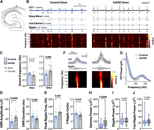
Figure 2.

SWRs are increased in three-month 5xFAD mice. A, SWRs were recorded in acute horizontal slices with the LFP electrode located in CA1. B, Example traces of three-month control (left) and 5xFAD (right) slices. First trace, LFP filtered between 1 and 1000 Hz, raster below indicates detected SWR events as overlap of SW and ripple events. Second trace, SW, filtered between 1 and 30 Hz, raster below indicates detected SW events. Third trace, Low γ, filtered between 20 and 50 Hz. Fourth trace, Ripple, filtered between 120 and 220 Hz, raster below indicates detected ripple events. Bottom, Z-scored time-frequency spectrogram from 1 to 250 Hz. C, Summary plot of SWR event frequency for 5xFAD and littermate controls for both one-month (n_mice = 10 CT, 10 5xFAD; left) and three-month cohorts (n_mice = 27 CT, 29 5xFAD; right). D, SWR event amplitude and duration. E, Peak ripple frequency and the number of ripple cycles within SWR duration. F, Example SWR events for traces displayed in B, with average z-scored time-frequency spectrogram of all events below. G, Average FFT of 200-ms window around all SWR events from characteristic subset of n_slice = 7 CT, 7 5xFAD from n_mice = 4 CT, 5 5xFAD. Shaded region represents SEM. H–J, SWR-locked oscillation power in the low γ (20–50 Hz; H), ripple (120–220 Hz; I), and fast ripple (250–500 Hz; J) ranges. Note that in H, one value was identified as an outlier by the ROUT method but was retained in analysis, as the data point appeared valid, and even with removal did not alter the observed increase (U = 193, p = 0.0015; Mann–Whitney). For all plots, individual data points represent the average of all slices recorded from an animal (n_slice/animal in Table 1). Closed circles represent males, open circles females. Bar plots indicate normal data with mean ± SEM. Box-whisker plots represent non-normal data with Median and IQRs; p values indicated above brackets.