Figure 5. Moffat functions provide a better description of axial intensity profiles than Gaussians.

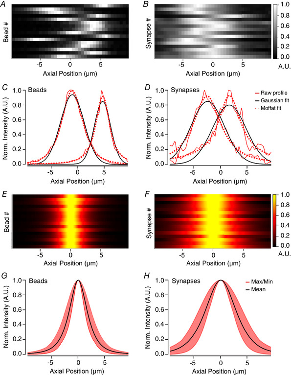
A and B, axial profiles for a selection of 16 fluorescent beads (A) or synapses (B) from a single field of view. Each row represents an ROI and has been normalised to the maximum for display purposes. C, raw axial profiles of 2 example beads (red lines), together with best‐fit Gaussian (black) and Moffat (red dotted) functions. For the left‐hand profile, Gaussian SD = 3.15 µm and Moffat function has α = 3.58 and β = 1.97. For right‐hand profile, Gaussian SD = 2.2 µm and Moffat function α = 1.9 and β = 1.35. Note that the peak and tails of the profile is underestimated by the Gaussian fit, but not the Moffat function. D, as in C but for 2 example synapses. For the left‐hand profile, Gaussian SD = 2.5 µm and Moffat function has α = 3.3 and β = 1.09. For right‐hand profile, Gaussian SD = 3.7 µm and Moffat function α = 1.7 and β = 0.49. Again, a Moffat function provides a better description than a Gaussian. E and F, fitted axial profiles of the same beads (E) and synapses (F) as in A and B with peaks realigned to the centre, showing the homogeneity of beads compared to synapses. G, average Moffat function fitted to profile of beads has α = 2.73 and β = 1.59 (black line). The red shaded area shows the variance. H, average Moffat function fitted to profile of synapses has α = 5.95 and β = 2.13 (black line).