A novel covid-19 mathematical model with fractional derivatives: Singular and nonsingular kernels

Abstract

In this paper, we considered a new mathematical model depicting the possibility of spread within a given general population. The model is constructed with five classes including susceptible, exposed, infected, recovered and deaths. We presented a detailed analysis of the suggested model including, the derivation of equilibrium points endemic and disease-free, reproductive number using the next generation matrix, the stability analysis of the equilibrium points and finally the positiveness of the model solutions. The model was extended to the concept of fractional differentiation to capture different memories including power law, decay and crossover behaviors. A numerical method based on the Newton was used to provide numerical solutions for different memories.

1. Introduction

Partial and ordinary differential equations have been used in many academic disciplines to model real world problems occurring in real life in daily [1], [3], [4]. They are wider used as they depict the variation or changes in time and space, thus they can be used together with many others parameters to model a given problems [2], [5]. We should note that these differential operators do not replicate exactly complex problems, however some can really replicate real world scenario especially those appearing in classical mechanic where the Markovian processes where the initial starting point and the generator operators are used to future in time and space. It is also important to note that a given real world problem can be modeled using different mathematical models especially when the variation of the real world problem is not well understood by modelers. In the last passed months, the world has faced an outbreak of a fatal disease called corona or covid-19, it is known that such virus comes from bats and was transmitted to humans. The virus has spread in all the corners of the globe and has taken the life of many humans around the world. The outbreak lead mankind in great panic, thus forced them to focus their attention to observe, analyze and predict the future outbreak of the disease, thus one will find many mathematical equations within the available literature many mathematical models [7], [8], [9], [10], [11]. However those mathematical models have their advantages and disadvantage, this is due to the fact that the spread or transmission of the disease is still not well understood by human. In this paper, a relatively new mathematical model and the concept of fractional differentiation and integration will be used to include into mathematical model more effects of non-localities.

2. Preliminaries

We present here useful definitions of fractional differential and integral operators. These operators will be used in the next section in order to include into mathematical formulation different effect of non-localities that could be exhibited by the spread of covid-19.

Definition 2.1

Let $f:R+\to R$ and $\beta \in (n-1,n),n\in N$. The left Caputo fractional derivative of order of the function f is given by the following equality;

$$C_0{D}_t\vartheta u\left(t\right)=\frac{1}{\Gamma (n-\vartheta )}{\int }_{0}t(t-y)n-\vartheta -1u\left(n\right)\left(y\right)dy.$$ (2.1)

Definition 2.2

The fractional integral associate to the new fractional integral with power-law kernel is defined as:

$$C_0{I}_t\vartheta u\left(t\right)=\frac{1}{\Gamma \left(\vartheta \right)}{\int }_{0}t(t-y)\vartheta -1u\left(y\right)dy.$$ (2.2)

Definition 2.3

Let u ∈ H ¹(a, b), b > a, ϑ ∈ [0, 1] then the new Caputo derivative of fractional order is given by:

$$D{\vartheta }_t\left(u\left(t\right)\right)=\frac{M\left(\vartheta \right)}{(1-\vartheta )}{\int }_{a}tu\prime \left(x\right)\exp [-\vartheta \frac{t-x}{1-\vartheta }]dx.$$ (2.3)

where M(ϑ) is a normalization function such that $M\left(0\right)=M\left(1\right)=1$ [6]. But, if the function u ≠ H ₁(a, b) then, new derivative called the Caputo-Fabrizio fractional derivative can be defined as

$$D{\vartheta }_t\left(u\left(t\right)\right)=\frac{M\left(\vartheta \right)}{(1-\vartheta )}{\int }_{a}t(u\left(t\right)-u\left(x\right))\exp [-\vartheta \frac{t-x}{1-\vartheta }]dx.$$ (2.4)

Definition 2.4

u ∈ H ¹(x, y), y > x, ϑ ∈ [0, 1] with the function f differentiable then, the definition of the new fractional derivative (Atangana-Baleanu derivative in Caputo sense) is given as

$${}_{a}ABCD{\vartheta }_t\left[u\left(t\right)\right]=\frac{B\left(\vartheta \right)}{1-\vartheta }{\int }_{a}t\frac{d}{dt}u\left(x\right)E_{\vartheta }[-\vartheta \frac{(t-x)\vartheta }{1-\vartheta }]dx.$$ (2.5)

where B(ϑ) has the same properties as in the case of the Caputo-Fabrizio fractional derivative.

Here $B\left(\vartheta \right)=1-\vartheta +\frac{\vartheta }{\Gamma \left(\vartheta \right)}.$

It should be noted that we do not recover the original function when $\vartheta =0$ except when at the origin the function vanishes. To avoid this kind of problem, the following definition is proposed.

Definition 2.5

Let u ∈ H ¹(x, y), y > x, ϑ ∈ [0, 1] and not necessary differentiable then, the definition of the new fractional derivative (Atangana-Baleanu fractional derivative in Riemann-Liouville sense) is given as [1].

$${}_{a}ABRD{\vartheta }_t\left[u\left(t\right)\right]=\frac{B\left(\vartheta \right)}{1-\vartheta }\frac{d}{dt}{\int }_{a}tu\left(x\right)E_{\vartheta }[-\vartheta \frac{(t-x)\vartheta }{1-\vartheta }]dx.$$ (2.6)

Definition 2.6

The fractional integral associate to the new fractional derivative with nonlocal kernel (Atangana-Baleanu fractional integral) is given as [1]:

$${}_{a}ABCI{\vartheta }_t\left[u\left(t\right)\right]=\frac{1-\vartheta }{B\left(\vartheta \right)}u\left(t\right)+\frac{\vartheta }{B\left(\vartheta \right)\Gamma \left(\vartheta \right)}{\int }_{a}tu\left(j\right)(t-j)\vartheta -1dj.$$ (2.7)

When alpha is zero we recover the initial function and if also alpha is 1, we obtain the ordinary integral.

3. Mathematical model

Although sometime mathematical models cannot replicate accurately the real world problem, of course due to that fact that the translation from real world observed problem to mathematical formula is not really accurate due to lack of information, or lack of accuracy to converting reality to mathematical formula. However, these models have been used in the last past decades with great success, thus their use is important to mankind for prediction. These prediction help human you have an idea of what could happen in near future, such that they can take some control measures to avoid worse case scenario. In this section therefore, we present a mathematical model, but simple, that could be used to predict the spread of covid-19 in a given population.

$$\begin{array}{cc}& \dot{S}\left(t\right)=-{\alpha }_{e}SE-{\alpha }_{i}SI+rR+\Lambda \hfill \\ & \dot{E}\left(t\right)={\alpha }_{e}SE+{\alpha }_{i}SI-KE-\phi E\hfill \\ & \dot{I}\left(t\right)=KE-\beta I-\mu I\hfill \\ & \dot{R}\left(t\right)=\beta I+\phi E-rR\hfill \\ & \dot{D}\left(t\right)=\mu I\hfill \end{array}$$ (3.1)

Here

• S(t) is the class of susceptible,

• E(t) is the class of expressed population

• I(t) is the infected class

• R(t) is the class of recovered,

• D(t) is the death clas

we present below the slandered analysis, that includes the first testing of disease-free equilibrium endemic-equilibrium, reproductive number, stability analysis.

This will be achieved by neglecting the death class, as such class does not give value to equilibrium.

For disease-free equilibrium we have

$$E_0=(0,0,0,0)$$

For endemic-equilibrium, we have

$$\begin{array}{cc}& -{\alpha }_e{S}^{*}{E}^{*}-{\alpha }_i{S}^{*}{I}^{*}+r{R}^{*}+\Lambda \hfill \\ & {\alpha }_e{S}^{*}{E}^{*}+{\alpha }_i{S}^{*}{I}^{*}-K{E}^{*}-\phi E^{*}=0\hfill \\ & K{E}^{*}-\beta I^{*}-\mu I^{*}=0\hfill \\ & \beta I^{*}+\phi E^{*}-r{R}^{*}=0\hfill \end{array}$$ (3.2)

$$\begin{array}{cc}& I^{*}={\displaystyle \frac{K}{\beta +\mu }}{E}^{*}\hfill \\ & R^{*}=({\displaystyle \frac{\beta K}{\beta +\mu }}+\phi )E^{*}\hfill \\ & S^{*}=\frac{K+\phi }{{\alpha }_i+\frac{{\alpha }_{i}K}{\beta +\mu }}\hfill \end{array}$$ (3.3)

$$\frac{\Lambda }{({\alpha }_i+{\alpha }_e)\left(\frac{K+\phi }{{\alpha }_i+\frac{{\alpha }_{i}K}{\beta +\mu }}\right)-(\frac{\beta K}{\beta +\mu }+\phi )}$$ (3.4)

Thus finally, we have

$$I^{*}=\frac{K}{\beta +\mu }\frac{\Lambda }{({\alpha }_i+{\alpha }_e)\left(\frac{K+\phi }{{\alpha }_i+\frac{{\alpha }_{i}K}{\beta +\mu }}\right)-(\frac{\beta K}{\beta +\mu }+\phi )}$$ (3.5)

$$R^{*}=(\frac{\beta K}{\beta +\mu }+\phi )\frac{\Lambda }{({\alpha }_i+{\alpha }_e)\left(\frac{K+\phi }{{\alpha }_i+\frac{{\alpha }_{i}K}{\beta +\mu }}\right)-(\frac{\beta K}{\beta +\mu }+\phi )}$$ (3.6)

$$S^{*}=\frac{K+\phi }{{\alpha }_i+\frac{{\alpha }_{i}K}{\beta +\mu }}$$ (3.7)

$$E^{*}=\frac{\Lambda }{({\alpha }_i+{\alpha }_e)\left(\frac{K+\phi }{{\alpha }_i+\frac{{\alpha }_{i}K}{\beta +\mu }}\right)-(\frac{\beta K}{\beta +\mu }+\phi )}$$ (3.8)

Now we deserve the reproductive number using the next generation matrix. To obtain this, we need only the following equations associate to the infection

$$\dot{E}\left(t\right)={\alpha }_{e}SE+{\alpha }_{i}SI-KE-\phi E$$ (3.9)

$$\dot{I}=KE-(\beta +\mu )I$$ (3.10)

$$F=\left(\begin{array}{cc}{\alpha }_{e}S& {\alpha }_{i}S\\ 0& 0\end{array}\right)$$ (3.11)

$$V=\left(\begin{array}{cc}-K+\phi & 0\\ -K& \beta +\mu \end{array}\right)$$ (3.12)

$$FV-1=\left(\begin{array}{cc}{\alpha }_{e}S& {\alpha }_{i}S\\ 0& 0\end{array}\right)\left(\begin{array}{cc}\frac{\beta +\mu }{(\beta +\mu )(K+\phi )}& 0\\ \frac{K}{(\beta +\mu )(K+\phi )}& \frac{\beta +\mu }{(\beta +\mu )(K+\phi )}\end{array}\right)$$ (3.13)

$$=\left(\begin{array}{cc}\frac{{\alpha }_{e}S}{K+\phi }+\frac{{\alpha }_{i}SK}{(\beta +\mu )(K+\phi )}& \frac{{\alpha }_{i}S}{\beta +\mu }\\ 0& 0\end{array}\right)$$ (3.14)

The reproductive number can be determined as

$$R_0=\frac{{\alpha }_{e}S(\beta +\mu )+{\alpha }_{i}SK}{(K+\phi )(\beta +\mu )}$$ (3.15)

Lemma 3.1

Lemma: There exist a unique endemic- equilibrium E* if R₀ > 1 and no endemic if $R_0=0$

Proof: To have endemic we need $\frac{d\dot{E}\left(t\right)}{dt}>0$ and $\frac{dI\left(t\right)}{dt}>0$ That is to say

$${\alpha }_{e}SE+{\alpha }_{i}SI-(K+\phi )E>0$$ (3.16)

$$KE-(\beta +\mu )I>0$$ (3.17)

$${\alpha }_{e}SE+{\alpha }_{i}SI>(K+\phi )E$$ (3.18)

$$\frac{{\alpha }_{e}SE+{\alpha }_{i}IS}{K+\phi }>E$$ (3.19)

with

$$I<\frac{KE}{\beta +\mu }$$ (3.20)

$$\frac{{\alpha }_{e}S+\frac{{\alpha }_{i}KS}{\beta +\mu }}{K+\phi }>1$$ (3.21)

$$\frac{{\alpha }_{e}S(\beta +\mu )+{\alpha }_{i}KS}{(k+\phi )(\beta +\mu )}>1$$ (3.22)

$$k_0>1$$ (3.23)

Thus there exists a unique endemic equilibrium if R ₀ > 1.

The Jacobian matrix associated to the system is given as

$$J=\left(\begin{array}{cccc}{\alpha }_{e}E-{\alpha }_{i}I& {\alpha }_{e}S& -{\alpha }_{i}S& r\\ {\alpha }_{e}E+{\alpha }_{i}I& -k-\phi +{\alpha }_{e}S& {\alpha }_{i}S& 0\\ 0& K& -\beta -\mu & 0\\ 0& \phi & \beta & -r\end{array}\right)$$ (3.24)

$$J\left(t^{*}\right)=\left(\begin{array}{cccc}0& 0& 0& r\\ 0& -k-\phi & 0& 0\\ 0& K& -\beta -\mu & 0\\ 0& \phi & \beta & -r\end{array}\right)$$ (3.25)

Here the trace is given as trace $\left(J\right(E0\left)\right)=-(K+\phi +\beta +\mu +r)<0\det \left(J\right(E0\left)\right)=0$

4. Global asymptotic stability

In this section, we present the analysis of global asymptotic stability. Using the two equations involving the primary infections, we insist the following Lyapunov

$$L=\frac{1}{K+\phi }E+\frac{1}{\beta +\mu }I$$ (4.1)

Thus applying the first derivative on both sides, we obtain

$$\begin{array}{cc}{\displaystyle \dot{L}}\hfill & {\displaystyle =\frac{1}{K+\phi }\dot{E}+\frac{1}{\beta +\mu }\dot{I}}\hfill \\ & {\displaystyle =\frac{1}{K+\phi }({\alpha }_{e}SE+{\alpha }_{i}SI-(K+\phi )E)+\frac{1}{\beta +\mu }(KE-(\beta +\mu )I)}\hfill \\ & {\displaystyle =\frac{1}{K+\phi }({\alpha }_{e}SE+{\alpha }_{i}SI)+\frac{KE}{\beta +\mu }-(E+I)}\hfill \\ & {\displaystyle =[((\frac{1}{K+\phi }({\alpha }_{e}SE+{\alpha }_{i}SI)+\frac{KE}{\beta +\mu })\frac{1}{E+I}-1](E+I)}\hfill \\ & {\displaystyle \ge [((\frac{1}{K+\phi }({\alpha }_{e}SE+{\alpha }_{i}SI)+\frac{KE}{\beta +\mu })\frac{1}{E+I}-1](E+I)}\hfill \\ & {\displaystyle \ge [\frac{{\alpha }_{e}S(\beta +\mu )+{\alpha }_{e}SK}{(K+\phi )(\beta +\mu )}-1](E+I)}\hfill \\ & {\displaystyle \ge (R_0-1)(E+I)}\hfill \end{array}$$ (4.2)

Thus

If R ₀ < 1, then $\frac{dL}{dt}<0$ if $\frac{dL}{dt}=0$ if $E=I=0$

5. Local and global stability of E*

In this section, we make use of the Jacobian matrix and the Lyapunov for endemic equilibrium. we start by the Jacobian matrix.

$$J=\left(\begin{array}{cccc}-{\alpha }_e{S}^{*}-{\alpha }_i{S}^{*}& {\alpha }_{e}S& -{\alpha }_{i}S& r\\ -{\alpha }_e{S}^{*}-{\alpha }_i{S}^{*}& -k-\phi +{\alpha }_{e}S& {\alpha }_{i}S& 0\\ 0& K& -\beta -\mu & 0\\ 0& \phi & \beta & -r\end{array}\right)$$ (5.1)

The characteristic equation associate to the above matrix can the obtained with

(5.2)

where I is the 4 × 4 identity matrix

$$\det \left(\begin{array}{cccc}\lambda +{\delta }_1& {\alpha }_e{S}^{*}& -{\alpha }_i{S}^{*}& r\\ {\delta }_1& \lambda +{\delta }_2& {\alpha }_i{S}^{*}& 0\\ 0& K& \lambda +{\delta }_3& 0\\ 0& \phi & \beta & \lambda +r\end{array}\right)$$ (5.3)

Thus

$$P_{J{E}^{*}}=\lambda 4+a_1\lambda 3+a_2\lambda 2+a_3\lambda +a_4$$ (5.4)

The Hurwitz matrix for the above characteristic polynomial equation is given as

$$H=\left(\begin{array}{cccc}{a}_1& a_3& 0& 0\\ 1& a_2& a_4& 0\\ 0& a_1& a_3& 0\\ 0& 1& a_2& a_4\end{array}\right)$$ (5.5)

$$H_1=a_1>0$$

$$H_2=a_1{a}_2-a_3>0$$

$$H_3=a_1{a}_2{a}_3-a_{1}2a_4-a_3>0$$

$$H_4=a_4{H}_3>0$$

we now prove the global asymptotic stability by using the Lyapunov function however the death class is excluded

$$\begin{array}{ccc}\hfill L& =& (S-S^{*}-S^{*}\log {\displaystyle \frac{S}{S^{*}}})+(E-E^{*}-E^{*}\log {\displaystyle \frac{E}{E^{*}}})\hfill \\ & & +(I-I^{*}-I^{*}\log \frac{I}{I^{*}})+(R-R^{*}-R^{*}\log {\displaystyle \frac{R}{R^{*}}})\hfill \end{array}$$ (5.6)

Thus the derivative respect to t is given as

$${\displaystyle \dot{L}=\left(\frac{S-S^{*}}{S}\right)\dot{S}+\left(\frac{I-I^{*}}{I}\right)\dot{I}+\left(\frac{E-E^{*}}{E}\right)\dot{E}+\left(\frac{R-R^{*}}{R}\right)\dot{R}}$$ (5.7)

$$\begin{array}{cc}& {\displaystyle =\left(\frac{R-R^{*}}{R}\right)(\beta I+\phi E-rR)+\left(\frac{I-I^{*}}{I}\right)(KE-(\beta +\mu )I)}\hfill \\ & {\displaystyle +({\alpha }_{e}SE+{\alpha }_{i}SI-(K+\phi )E)+\left(\frac{S-S^{*}}{S}\right)(-{\alpha }_{e}SE-{\alpha }_{i}SI+rR+\Lambda )}\hfill \end{array}$$ (5.8)

$$\begin{array}{cc}\dot{L}\hfill & {\displaystyle \ge \left(\frac{R-R^{*}}{R}\right)(\beta (I-I^{*})+\phi (E-E^{*})-r(R-R^{*}))}\hfill \\ & {\displaystyle +\left(\frac{I-I^{*}}{I}\right)(K(E-E^{*})-(\beta +\mu )(I-I^{*}))}\hfill \\ & {\displaystyle +\left(\frac{E-E^{*}}{E}\right)({\alpha }_e(S-S^{*})(E-E^{*})+{\alpha }_i(S-S^{*})(I-I^{*})-(K+\phi )(E-E^{*})}\hfill \\ & {\displaystyle +\left(\frac{S-S^{*}}{S}\right)(-{\alpha }_e(S-S^{*})(E-E^{*})-{\alpha }_i(S-S^{*})(I-I^{*})+r(R-R^{*})+\Lambda )}\hfill \end{array}$$ (5.9)

$$\begin{array}{cc}\ge \hfill & {\displaystyle -r\frac{(R-R^{*})2}{R}+\beta I-\beta I^{*}+\phi E-\phi E^{*}}\hfill \\ & {\displaystyle -\frac{R^{*}}{R}\beta I+\frac{R^{*}}{R}\beta I^{*}-\phi E\frac{R^{*}}{R}+\phi E^{*}\frac{R^{*}}{R}}\hfill \\ & {\displaystyle -(\beta +\mu )\frac{(I-I^{*})2}{I}+KE-K{E}^{*}-\frac{I^{*}}{I}KE+\frac{I^{*}}{I}K{E}^{*}+\frac{(E-E^{*})2}{E}{\alpha }_{e}S}\hfill \\ & {\displaystyle -{\alpha }_e\frac{(E-E^{*})2}{E}{S}^{*}-(K+\phi )\frac{(E-E^{*})2}{E}+{\alpha }_{i}SI-{\alpha }_{i}S{I}^{*}-{\alpha }_i{S}^{*}I+{\alpha }_i{S}^{*}{I}^{*}}\hfill \\ & {\displaystyle -{\alpha }_{i}SI\frac{E^{*}}{E}+{\alpha }_{i}S{I}^{*}\frac{E^{*}}{E}+{\alpha }_i{S}^{*}I\frac{E^{*}}{E}-{\alpha }_i{S}^{*}{I}^{*}\frac{E^{*}}{E}-{\alpha }_e\frac{(S-S^{*})2}{S}E}\hfill \\ & {\displaystyle +{\alpha }_e{E}^{*}\frac{(S-S^{*})2}{S}-{\alpha }_i\frac{(S-S^{*})2}{S}I+{\alpha }_i\frac{(S-S^{*})2}{S}{I}^{*}+rR-rR*+\Lambda }\hfill \\ & {\displaystyle -\frac{S^{*}}{S}rR+r\frac{R^{*}{S}^{*}}{S}-\Lambda \frac{S}{S^{*}}}\hfill \end{array}$$ (5.10)

$$\begin{array}{cc}\ge \hfill & {\displaystyle \beta I+\phi E^{*}+\frac{R^{*}}{R}\beta I^{*}+\phi E^{*}\frac{R^{*}}{R}+KE+\frac{I^{*}}{I}K{E}^{*}+\frac{(E-E^{*})2}{E}+{\alpha }_{i}SI+{\alpha }_i{S}^{*}{I}^{*}}\hfill \\ & {\displaystyle +{\alpha }_{i}S{I}^{*}\frac{E^{*}}{E}+{\alpha }_i{S}^{*}I\frac{E^{*}}{E}+{\alpha }_{i}E\frac{(S-S^{*})2}{S}+{\alpha }_i\frac{(S-S^{*})2}{I}{I}^{*}+rR}\hfill \\ & {\displaystyle +\Lambda +r{R}^{*}\frac{S^{*}}{S}+\Lambda \frac{S^{*}}{S}-(\frac{r(R-R^{*})2}{R}+\beta I^{*}+\phi E^{*}\beta I\frac{R^{*}}{R}+\phi E\frac{R^{*}}{R}+(\beta +\mu )}\hfill \\ & {\displaystyle +\frac{(I-I^{*})2}{I}+K{E}^{*}+\frac{I^{*}}{I}KE+{\alpha }_e\frac{(E-E^{*})2}{E}{S}^{*}+(K+\phi )+\frac{(E-E^{*})2}{E}}\hfill \\ & {\displaystyle +{\alpha }_{i}S{I}^{*}+{\alpha }_i{S}^{*}I}\hfill \\ & {\displaystyle +{\alpha }_{i}SI\frac{E^{*}}{E}+{\alpha }_i{S}^{*}{I}^{*}\frac{E^{*}}{E}+{\alpha }_i{S}^{*}{I}^{*}\frac{E^{*}}{E}+{\alpha }_e\frac{(S-S^{*})2}{S}E+{\alpha }_i\frac{(S-S^{*})2}{S}}\hfill \\ & {\displaystyle +r{R}^{*}+rR\frac{S^{*}}{S}+\Lambda \frac{S^{*}}{S})}\hfill \end{array}$$ (5.11)

$$\ge A-B$$

Therefore $\frac{dL}{dt}>0$ if $A-B>0$

$\frac{dL}{dt}=0$ if $A=B$ and $\frac{dL}{dt}<0$ if $A-B<0.$

6. Positive solutions

Differential operators defined as convolution of classical differential operators and kernel including power law, exponential decay function and the generalized Mittag-Leffler function have abilities to include into mathematical equations the effect of power law, fading memory and behaviors with crossover properties. Due to uncertainties around the spread of covid-19, we will use such differential operators to have more possibilities of spread. Thus in this section, we convert the classical differential operator to fractional counterpart.

Since the suggested Mathematical model predict the behavior of real world problem where the solutions represent positive numbers, we shall prove that ∀t ≥ 0, all the solutions are positives for all 3 cases of fractional derivatives. We start with Caputo-Fabrizio case,

$$\begin{array}{cc}& {}_{0}CFD{\vartheta }_{t}S\left(t\right)=-{\alpha }_{e}SE-{\alpha }_{i}SI+rR+\Lambda \hfill \\ & {}_{0}CFD{\vartheta }_{t}E\left(t\right)={\alpha }_{e}SE+{\alpha }_{i}SI-KE-\phi E\hfill \\ & {}_{0}CFD{\vartheta }_{t}I\left(t\right)=KE-\beta I-\mu I\hfill \\ & {}_{0}CFD{\vartheta }_{t}R\left(t\right)=\beta I+\phi E-rR\hfill \\ & {}_{0}CFD{\vartheta }_{t}D\left(t\right)=\mu I\hfill \end{array}$$ (6.1)

we use the as yune. used by [11] where the suggested that all the product of two different classes should positive thus

$$\begin{array}{cc}{}_{0}CFD{\vartheta }_{t}E\left(t\right)\hfill & =-{\alpha }_{e}SE-{\alpha }_{i}SI-(K+\phi )E\hfill \\ & \ge -(K+\phi )E\hfill \end{array}$$ (6.2)

$$E\left(t\right)\ge E\left(0\right)\exp [-\frac{\vartheta (K+\phi )t}{M\left(\vartheta \right)-(1-\vartheta )(K+\phi )}]\forall t>0$$ (6.3)

$$\begin{array}{cc}& {}_{0}CFD{\vartheta }_{t}R\left(t\right)=\beta I+\phi E-rR\hfill \\ & -rR\hfill \end{array}$$ (6.4)

$$R\left(t\right)\ge R\left(0\right)\exp [-\frac{\vartheta rt}{M\left(\vartheta \right)-(1-\vartheta )r}]\forall t>0.$$ (6.5)

$$\begin{array}{cc}{}_{0}CFD{\vartheta }_{t}I\left(t\right)\hfill & =KE-(\beta +\mu )I\hfill \\ & -(\beta +\mu )I\hfill \end{array}$$ (6.6)

$$I\left(t\right)\ge I\left(0\right)\exp [-\frac{\vartheta (\beta +\mu )t}{M\left(\vartheta \right)-(1-\vartheta )r(\beta +\mu )}]$$ (6.7)

Since I(t)    ∀t ≥ 0 thus

$$\begin{array}{cc}D\left(t\right)\hfill & ={\displaystyle \frac{(1-\vartheta )\mu I\left(t\right)}{M\left(\vartheta \right)}}+{\displaystyle \frac{\vartheta \mu }{M\vartheta }}{\int }_{0}tI\left(t\right)d\tau \hfill \\ & \ge 0\forall t\ge 0\hfill \end{array}$$ (6.8)

$$\begin{array}{cc}{}_{0}CFD{\vartheta }_{t}S\left(t\right)\hfill & =-{\alpha }_{e}SE-{\alpha }_{i}SI+rR+\Lambda \hfill \\ & \ge -S(E+I)\hfill \\ & -S\left(\right|E|+|I\left|\right)\hfill \\ & \ge -S\left(t\right)\left(\underset{t\in D_E}{\sup }\right|E|+\underset{t\in D_I}{\sup }|I\left(t\right)\left|\right)\hfill \\ & -S\left(t\right)({\left|E\right|}_{\infty }+{\left|I\right|}_{\infty })\hfill \\ & \ge -S\left(t\right)\mathcal{M}\hfill \\ & \ge S\left(0\right)\exp [-\frac{\vartheta \mathcal{M}t}{\mathcal{M}\left(\vartheta \right)-(1-\vartheta )\mathcal{M}}]\hfill \end{array}$$ (6.9)

with power law kernel we have

$$\begin{array}{cc}& {}_{0}CD{\vartheta }_{t}S\left(t\right)=-{\alpha }_{e}SE-{\alpha }_{i}SI+rR+\Lambda \hfill \\ & {}_{0}CD{\vartheta }_{t}E\left(t\right)={\alpha }_{e}SE+{\alpha }_{i}SI-KE-\phi E\hfill \\ & {}_{0}CD{\vartheta }_{t}I\left(t\right)=KE-\beta I-\mu I\hfill \\ & {}_{0}CD{\vartheta }_{t}R\left(t\right)=\beta I+\phi E-rR\hfill \\ & {}_{0}CD{\vartheta }_{t}D\left(t\right)=\mu I\hfill \end{array}$$ (6.10)

we did before, we have

$$\begin{array}{cc}& S\left(t\right)\ge S\left(0\right)E_{\vartheta }[-\mathcal{M}t\vartheta ]\forall t\ge 0\hfill \\ & E\left(t\right)\ge E\left(0\right)E_{\vartheta }[-(K+\phi )t\vartheta ]\forall t\ge 0\hfill \\ & I\left(t\right)\ge I\left(0\right)E_{\vartheta }[-(\beta +\mu )t\vartheta ]\forall t\ge 0\hfill \\ & R\left(t\right)\ge R\left(0\right)E_{\vartheta }[-rt\vartheta ]\forall t\ge 0\hfill \end{array}$$ (6.11)

$$D\left(t\right)=\frac{\mathcal{M}}{I\left(\vartheta \right)}{\int }_{0}tI\left(\tau \right)(t-\tau )\vartheta -1d\tau \forall t\ge 0$$ (6.12)

with Atangana-Baleanu fractional derivative

$$\begin{array}{cc}& {}_{0}ABCD{\vartheta }_{t}S\left(t\right)=-{\alpha }_{e}SE-{\alpha }_{i}SI+rR+\Lambda \hfill \\ & {}_{0}ABCD{\vartheta }_{t}E\left(t\right)={\alpha }_{e}SE+{\alpha }_{i}SI-KE-\phi E\hfill \\ & {}_{0}ABCD{\vartheta }_{t}I\left(t\right)=KE-\beta I-\mu I\hfill \\ & {}_{0}ABCD{\vartheta }_{t}R\left(t\right)=\beta I+\phi E-rR\hfill \\ & {}_{0}ABCD{\vartheta }_{t}D\left(t\right)=\mu I\hfill \end{array}$$ (6.13)

Thus using the same routine

$$I\left(t\right)\ge I\left(0\right)E_{\vartheta }[-\frac{(\beta +\mu )t\vartheta }{AB\left(\vartheta \right)-(1-\vartheta )(\beta +\mu )}]$$ (6.14)

$$E\left(t\right)\ge E\left(0\right)E_{\vartheta }[-\frac{(K+\phi )t\vartheta }{AB\left(\vartheta \right)-(1-\vartheta )(K+\phi )}]$$ (6.15)

$$S\left(t\right)\ge S\left(0\right)S_{\vartheta }[-\frac{\left(\mathcal{M}\right)t\vartheta }{AB\left(\vartheta \right)-(1-\vartheta )\mathcal{M}}]$$ (6.16)

$$R\left(t\right)\ge R\left(0\right)R_{\vartheta }[-\frac{-rt\vartheta }{AB\left(\vartheta \right)-(1-\vartheta )r}]$$ (6.17)

$$\begin{array}{ccc}\hfill D\left(t\right)& =& \frac{(1-\vartheta )}{AB\left(\vartheta \right)}\mathcal{M}I\left(t\right)+\frac{\vartheta \mathcal{M}}{AB\left(\vartheta \right)\Gamma \left(\vartheta \right)}\hfill \\ & & \times {\int }_{0}tI\left(\tau \right)(t-\tau )\vartheta -1d\tau \forall t\ge 0\hfill \end{array}$$ (6.18)

7. Numerical method for Caputo-Fabrizio fractional derivative

In this section, we handle the following Cauchy problem with Caputo-Fabrizio fractional derivative

$$\begin{array}{c}\{\begin{array}{cc}& {}_{0}CFD{\vartheta }_{t}y\left(t\right)=f(t,y\left(t\right)),\hfill \\ & y\left(0\right)=y_0\hfill \end{array}\hfill \end{array}$$ (7.1)

where the function f is non-linear. To present a numerical scheme for solution of our equation, we can reformulate the above equation as

$$y\left(t\right)-y\left(0\right)=\frac{1-\vartheta }{M\left(\vartheta \right)}f(t,y\left(t\right))+\frac{\vartheta }{M\left(\Theta \right)}{\int }_{0}tf(\tau ,y\left(\tau \right))d\tau .$$ (7.2)

At the point $t_{n+1}=(n+1)\Delta t,$ we have

$$y\left(t_{n+1}\right)-y\left(0\right)=\frac{1-\vartheta }{M\left(\vartheta \right)}f(t_n,y\left(t_n\right))+\frac{\vartheta }{M\left(\vartheta \right)}{\int }_0{t}_{n+1}f(\tau ,y\left(\tau \right))d\tau .$$ (7.3)

at the point $t_n=n\Delta t,$ we have

$$y\left(t_n\right)-y\left(0\right)=\frac{1-\vartheta }{M\left(\vartheta \right)}f(t_{n-1},y\left(t_{n-1}\right))+\frac{\vartheta }{M\left(\vartheta \right)}{\int }_0{t}_{n}f(\tau ,y\left(\tau \right))d\tau .$$ (7.4)

If we take the difference of this equations, we obtain

$$\begin{array}{cc}y\left(t_{n+1}\right)-y\left(t_n\right)\hfill & ={\displaystyle \frac{1-\vartheta }{M\left(\vartheta \right)}}[f(t_n,y\left(t_n\right))-f(t_{n-1},y\left(t_{n-1}\right))]\hfill \\ & +{\displaystyle \frac{\vartheta }{M\left(\alpha \right)}}{\int }_{t_n}{t}_{n+1}f(\tau ,y\left(\tau \right))d\tau .\hfill \end{array}$$ (7.5)

and

$$\begin{array}{cc}y\left(t_{n+1}\right)-y\left(t_n\right)\hfill & ={\displaystyle \frac{1-\vartheta }{M\left(\vartheta \right)}}[f(t_n,y\left(t_n\right))-f(t_{n-1},y\left(t_{n-1}\right))]\hfill \\ & +{\displaystyle \frac{\vartheta }{M\left(\vartheta \right)}}\sum _{j=2}n{\int }_{t_j}{t}_{j+1}f(\tau ,y\left(\tau \right))d\tau .\hfill \end{array}$$ (7.6)

Using the Newton polynomial, we can write the approximation of the function f(t, y(t)) as follows

$$\begin{array}{cc}{P}_n\left(\tau \right)\hfill & =f(t_{n-2},y\left(t_{n-2}\right))+{\displaystyle \frac{f(t_{n-1},y\left(t_{n-1}\right))-f(t_{n-2},y\left(t_{n-2}\right))}{\Delta \left(t\right)}}\hfill \\ & (\tau -t_{n-2}){\displaystyle \frac{f(t_n,y\left(t_n\right))-2f(t_{n-1},y\left(t_{n-1}\right))+f(t_{n-2},y\left(t_{n-2}\right))}{2\left(\Delta t\right)2}}\hfill \\ & \times (\tau -t_{n-2})(\tau -t_{n-1}).\hfill \end{array}$$ (7.7)

Thus putting this polynomial into the above equation, we write the following

$$\begin{array}{cc}yn+1-yn\hfill & ={\displaystyle \frac{1-\vartheta }{M\left(\vartheta \right)}}[f(t_n,y\left(t_n\right))-f(t_{n-1},y\left(t_{n-1}\right))]\hfill \\ & +{\displaystyle \frac{\vartheta }{M\left(\vartheta \right)}}\sum _{j=2}n{\int }_{t_j}{t}_{j+1}\hfill \\ & \left\{\begin{array}{c}+f(t_{j-2},yj-2)\\ +\frac{f(t_{j-1},yj-1)-f(t_{j-2},yj-2)}{\Delta t}(\tau -t_{j-2})\\ +\frac{f(t_j,yj)-2f(t_{j-1},yj-1)+f(t_{j-2},yj-2)}{2\left(\Delta t\right)2}\\ \times (\tau -t_{j-2})(\tau -t_{j-1})\end{array}\right\}d\tau .\hfill \end{array}$$ (7.8)

and reorder as follows

$$\begin{array}{cc}yn+1-yn\hfill & ={\displaystyle \frac{1-\vartheta }{M\left(\vartheta \right)}}[f(t_n,y\left(t_n\right))-f(t_{n-1},y\left(t_{n-1}\right))]\hfill \\ & +{\displaystyle \frac{\vartheta }{M\left(\vartheta \right)}}\sum _{j=2}n{\int }_{t_j}{t}_{j+1}\hfill \\ & \left\{\begin{array}{cc}& +f(t_{j-2},yj-2)\\ & +\frac{f(t_{j-1},yj-1)-f(t_{j-2},yj-2)}{\Delta t}{\int }_{t_j}{t}_{j+1}(\tau -t_{j-2})d\tau \\ & +\frac{f(t_j,yj)-2f(t_{j-1},yj-1)+f(t_{j-2},yj-2)}{2\left(\Delta t\right)2}\\ & \times {\int }_{t_j}{t}_{j+1}(\tau -t_{j-2})(\tau -t_{j-1})d\tau \end{array}\right\}.\hfill \end{array}$$ (7.9)

We can have the following calculations for the above integrals

$${\int }_{t_j}{t}_{j+1}(\tau -t_{j-2})d\tau =\frac{5}{2}\left(\Delta t\right)2$$ (7.10)

$${\int }_{t_j}{t}_{j+1}(\tau -t_{j-2})(\tau -t_{j-1})d\tau =\frac{23}{6}\left(\Delta t\right)3$$ (7.11)

If we replace them into above scheme, we obtain the following scheme

$$\begin{array}{cc}yn+1\hfill & =yn+{\displaystyle \frac{1-\vartheta }{M\left(\vartheta \right)}}[f(t_n,y\left(t_n\right))-f(t_{n-1},y\left(t_{n-1}\right))]\hfill \\ & +{\displaystyle \frac{\vartheta }{M\left(\vartheta \right)}}\sum _{n}n=2\hfill \\ & \left\{\begin{array}{cc}& +f(t_{j-2},yj-2)\Delta t+[f(t_{j-1},yj-1)-f(t_{j-2},yj-2)]\frac{5}{2}\Delta t\\ & +[f(t_j,yj)-2f(t_{j-1},yj-1)+f(t_{j-2},yj-2)\frac{23}{6}\Delta t\end{array}\right\}.\hfill \end{array}$$ (7.12)

and we can rearrange as

$$\begin{array}{cc}yn+1\hfill & =yn+{\displaystyle \frac{1-\vartheta }{M\left(\vartheta \right)}}[f(t_n,y\left(t_n\right))-f(t_{n-1},y\left(t_{n-1}\right))]\hfill \\ & {\displaystyle +{\displaystyle \frac{\vartheta }{M\left(\vartheta \right)}}\sum _{n}n=2\{-\frac{4}{3}f(t_{j-1},yj-1)\Delta t+\frac{5}{12}f(t_{j-2},yj-2)\Delta t}\hfill \\ & +{\displaystyle \frac{23}{12}}f(t_j,yj)\Delta t\}\hfill \end{array}$$ (7.13)

8. Numerical method for Atangana-Baleanu fractional derivative

Now we deal with the following Cauchy problem with AtanganaâBaleanu fractional derivative

$$\begin{array}{c}\{\begin{array}{cc}& {}_{0}ABCD{\vartheta }_{t}y\left(t\right)=f(t,y\left(t\right)),\hfill \\ & y\left(0\right)=y_0\hfill \end{array}\hfill \end{array}$$ (8.1)

In this section, we provide a numerical scheme to solve this equation. Applying Atangana-Baleanu integral, we convert the above equation into

$$\begin{array}{ccc}\hfill y\left(t\right)-y\left(0\right)& =& \frac{1-\vartheta }{AB\left(\vartheta \right)}f(t,y\left(t\right))+\frac{\vartheta }{AB\left(\vartheta \right)\Gamma \left(\vartheta \right)}\hfill \\ & & \times {\int }_{0}tf(\tau ,y\left(\tau \right))(t-\tau )\vartheta -1d\tau .\hfill \end{array}$$ (8.2)

At the point $t_{n+1}=(n+1)\Delta t,$ we have

$$\begin{array}{ccc}\hfill y\left(t_{n+1}\right)-y\left(0\right)& =& \frac{1-\vartheta }{AB\left(\vartheta \right)}f(t_n,y\left(t_n\right))+\frac{\vartheta }{AB\left(\vartheta \right)\Gamma \left(\vartheta \right)}\hfill \\ & & \times {\int }_0{t}_{n+1}f(\tau ,y\left(\tau \right))(t_{n+1}-\tau )\vartheta -1d\tau .\hfill \end{array}$$ (8.3)

at the point $t_n=n\Delta t,$ we have

$$\begin{array}{ccc}\hfill y\left(t_{n+1}\right)-y\left(0\right)& =& \frac{1-\vartheta }{AB\left(\vartheta \right)}f(t_n,y\left(t_n\right))+\frac{\vartheta }{AB\left(\vartheta \right)\Gamma \left(\vartheta \right)}\sum _{j=2}n\hfill \\ & & \times {\int }_j{t}_{j+1}f(\tau ,y\left(\tau \right))d\tau .\hfill \end{array}$$ (8.4)

Here, for the approximation of the function f(t, y(t)), we use the Newton polynomial which is given by

$$\begin{array}{cc}{P}_n\left(\tau \right)\hfill & =f(t_{n-2},y\left(t_{n-2}\right))+{\displaystyle \frac{f(t_{n-1},y\left(t_{n-1}\right))-f(t_{n-2},y\left(t_{n-2}\right))}{\Delta \left(t\right)}}\hfill \\ & (\tau -t_{n-2}){\displaystyle \frac{f(t_n,y\left(t_n\right))-2f(t_{n-1},y\left(t_{n-1}\right))+f(t_{n-2},y\left(t_{n-2}\right))}{2\left(\Delta t\right)2}}\hfill \\ & \times (\tau -t_{n-2})(\tau -t_{n-1}).\hfill \end{array}$$ (8.5)

Thus if we write this polynomial in (8.4), we have the following

$$\begin{array}{cc}yn+1\hfill & =y0+{\displaystyle \frac{1-\vartheta }{AB\left(\vartheta \right)}}f(t_n,y\left(t_n\right))\hfill \\ & +{\displaystyle \frac{\vartheta }{AB\left(\vartheta \right)\Gamma \left(\vartheta \right)}}\sum _{j=2}n{\int }_{t_j}{t}_{j+1}\hfill \\ & \left\{\begin{array}{c}+f(t_{j-2},yj-2)\\ +\frac{f(t_{j-1},yj-1)-f(t_{j-2},yj-2)}{\Delta t}(\tau -t_{j-2})\\ +\frac{f(t_j,yj)-2f(t_{j-1},yj-1)+f(t_{j-2},yj-2)}{2\left(\Delta t\right)2}\\ \times (\tau -t_{j-2})(\tau -t_{j-1})\end{array}\right\}(t_{n+1}-\tau )\vartheta -1d\tau .\hfill \end{array}$$ (8.6)

and we can reorganize

$$\begin{array}{cc}yn+1\hfill & =y0+{\displaystyle \frac{1-\vartheta }{AB\left(\vartheta \right)}}f(t_n,y\left(t_n\right))\hfill \\ & +{\displaystyle \frac{\vartheta }{AB\left(\vartheta \right)\Gamma \left(\vartheta \right)}}\sum _{j=2}n\hfill \\ & \left\{\begin{array}{c}+{\int }_{t_j}{t}_{j+1}f(t_{j-2},yj-2)(t_{n+1}-\tau )\vartheta -1d\tau \\ +{\int }_{t_j}{t}_{j+1}\frac{f(t_{j-1},yj-1)-f(t_{j-2},yj-2)}{\Delta t}(\tau -t_{j-2})(t_{n+1}-\tau )\vartheta -1d\tau \\ +{\int }_{t_j}{t}_{j+1}\frac{f(t_j,yj)-2f(t_{j-1},yj-1)+f(t_{j-2},yj-2)}{2\left(\Delta t\right)2}\\ \times (\tau -t_{j-2})(\tau -t_{j-1})(t_{n+1}-\tau )\vartheta -1d\tau \end{array}\right\}.\hfill \end{array}$$ (8.7)

Thus we have

$$\begin{array}{cc}yn+1\hfill & {\displaystyle =y0+\frac{1-\vartheta }{AB\left(\vartheta \right)}f(t_n,y\left(t_n\right))}\hfill \\ & {\displaystyle +\frac{\vartheta }{AB\left(\vartheta \right)\Gamma \left(\vartheta \right)}\sum _{j=2}nf(t_{j-2},yj-2)\Delta t{\int }_{t_j}{t}_{j+1}(t_{n+1}-\tau )\vartheta -1d\tau }\hfill \\ & {\displaystyle +\frac{\vartheta }{AB\left(\vartheta \right)\Gamma \left(\vartheta \right)}\sum _{j=2}n\frac{f(t_{j-1},yj-1)-f(t_{j-2},yj-2)}{\Delta t}}\hfill \\ & {\displaystyle \times {\int }_{t_j}{t}_{j+1}(\tau -t_{j-2})(\tau -t_{j-1})(t_{n+1}-\tau )\vartheta -1d\tau }\hfill \\ & {\displaystyle +\frac{\vartheta }{AB\left(\vartheta \right)\Gamma \left(\vartheta \right)}\sum _{j=2}n\frac{f(t_j,yj)-2f(t_{j-1},yj-1)+f(t_{j-2},yj-2)}{2\left(\Delta t\right)2}}\hfill \\ & {\displaystyle \times {\int }_{t_j}{t}_{j+1}(\tau -t_{j-2})(\tau -t_{j-1})(t_{n+1}-\tau )\vartheta -1d\tau .}\hfill \end{array}$$ (8.8)

When calculating the above integrals

$$\begin{array}{cc}& {\int }_{t_j}{t}_{j+1}(t_{n+1}-\tau )\vartheta -1d\tau ={\displaystyle \frac{\left(\Delta t\right)\vartheta }{\vartheta }}[(n-j+1)\vartheta -(n-j)\vartheta ]\hfill \\ & {\int }_{t_j}{t}_{j+1}(\tau -t_{j-2})(t_{n+1}-\tau )\vartheta -1d\tau ={\displaystyle \frac{\left(\Delta t\right)\vartheta +1}{\vartheta (\vartheta +1)}}\hfill \\ & \left[\begin{array}{cc}& \hfill (n-j+1)\vartheta (n-j+3+2\vartheta )\\ & \hfill -(n-j)\vartheta (n-j+3+3\vartheta )\end{array}\right]\hfill \\ & {\int }_{t_j}{t}_{j+1}(\tau -t_{j-2})(\tau -t_{j-1})(t_{n+1}-\tau )\vartheta -1d\tau ={\displaystyle \frac{\left(\Delta t\right)\vartheta +2}{\vartheta (\vartheta +1)(\vartheta +2)}}\hfill \\ & \times \left[\begin{array}{cc}& \hfill (n-j+1)\vartheta \left[\begin{array}{cc}& \hfill 2(n-j)2+\left(3\vartheta +10\right)(n-j)\\ & \hfill +2\vartheta 2+9\vartheta +12\end{array}\right]\\ \hfill & \hfill -(n-j)\vartheta \left[\begin{array}{cc}& \hfill 2(n-j)2+(5\vartheta +10)(n-j)\\ & \hfill 6\vartheta 2+18\vartheta +12\end{array}\right]\end{array}\right]\hfill \end{array}$$ (8.9)

and putting this equalities into above scheme, we can obtain the following scheme

$$\begin{array}{cc}yn+1\hfill & {\displaystyle =y0+\frac{1-\vartheta }{AB\left(\vartheta \right)}f(t_n,y\left(t_n\right))}\hfill \\ & {\displaystyle +\frac{\vartheta \left(\Delta t\right)\vartheta }{AB\left(\vartheta \right)\Gamma (\vartheta +1)}\sum _{j=2}nf(t_{j-2},yj-2)[(n-j+1)\vartheta -(n-j)\vartheta ]}\hfill \\ & {\displaystyle +\frac{\vartheta \left(\Delta t\right)\vartheta }{AB\left(\vartheta \right)\Gamma (\vartheta +2)}\sum _{j=2}nf(t_{j-1},yj-1)-f(t_{j-2},yj-2)}\hfill \\ & {\displaystyle \times \left[\begin{array}{cc}& \hfill (n-j+1)\vartheta (n-j+3+2\vartheta )\\ & \hfill {\displaystyle -(n-j)\vartheta (n-j+3+3\vartheta )}\end{array}\right]}\hfill \\ & {\displaystyle +\frac{\vartheta \left(\Delta t\right)\vartheta }{AB\left(\vartheta \right)\Gamma (\vartheta +3)}\sum _{j=2}nf(t_j,yj)-2f(t_{j-1},yj-1)+f(t_{j-2},yj-2)}\hfill \\ & {\displaystyle \times \left[\begin{array}{cc}& \hfill (n-j+1)\vartheta \left[\begin{array}{cc}& \hfill 2(n-j)2+\left(3\vartheta +10\right)(n-j)\\ & \hfill {\displaystyle +2\vartheta 2+9\vartheta +12}\end{array}\right]\\ \hfill & \hfill -(n-j)\vartheta \left[\begin{array}{cc}& \hfill 2(n-j)2+(5\vartheta +10)(n-j)\\ & \hfill {\displaystyle 6\vartheta 2+18\vartheta +12}\end{array}\right]\end{array}\right].}\hfill \end{array}$$ (8.10)

9. Application to corona model with Caputo-Fabrizio and Atangana-Baleanu fractional derivative

In this section, we apply the differential and integral operators to the suggested mathematical model of COVID-19. Here, the classical differential operator will be replaced by the Caputo-Fabrizio and Atangana-Baleanu fractional derivative.

For simplicity, we write above equation (6.1) as follows;

$$\begin{array}{cc}& {}_{0}CFD{\vartheta }_t\dot{S}\left(t\right)=S_1(t,S,E,I,R,D)\hfill \\ & {}_{0}CFD{\vartheta }_t\dot{E}\left(t\right)=E_1(t,S,E,I,R,D)\hfill \\ & {}_{0}CFD{\vartheta }_t\dot{I}\left(t\right)=I_1(t,S,E,I,R,D)\hfill \\ & {}_{0}CFD{\vartheta }_t\dot{R}\left(t\right)=R_1(t,S,E,I,R,D)\hfill \\ & {}_{0}CFD{\vartheta }_t\dot{D}\left(t\right)=D_1(t,S,E,I,R,D)\hfill \end{array}$$ (9.1)

where

$$\begin{array}{cc}& S_1(t,S,E,I,R,D)=-{\alpha }_{e}SE-{\alpha }_{i}SI+rR+\Lambda \hfill \\ & E_1(t,S,E,I,R,D)={\alpha }_{e}SE+{\alpha }_{i}SI-KE-\phi E\hfill \\ & I_1(t,S,E,I,R,D)=KE-\beta I-\mu I\hfill \\ & R_1(t,S,E,I,R,D)=\beta I+\phi E-rR\hfill \\ & D_1(t,S,E,I,R,D)=\mu I\hfill \end{array}$$ (9.2)

After applying Caputo-Fabrizio fractional derivative we have the following

We can have the following scheme for this model

$$\begin{array}{cc}S\left(t_{n+1}\right)\hfill & =S\left(t_n\right)+{\displaystyle \frac{1-\vartheta }{M\left(\vartheta \right)}}[S_1(t_n,S\left(t_n\right),E\left(t_n\right),I\left(t_n\right),R\left(t_n\right),D\left(t_n\right))\hfill \\ & -S_1(t_{n-1},S\left(t_{n-1}\right),E\left(t_{n-1}\right),I\left(t_{n-1}\right),R\left(t_{n-1}\right),D\left(t_{n-1}\right))]\hfill \\ & +{\displaystyle \frac{\vartheta }{M\left(\vartheta \right)}}\sum _{n}n=2\{-\frac{4}{3}{S}_1(t_{n-1},S\left(t_{n-1}\right),E\left(t_{n-1}\right),I\left(t_{n-1}\right),R\left(t_{n-1}\right),D\left(t_{n-1}\right))\Delta t\hfill \\ & +\frac{5}{12}{S}_1(t_{n-2},S\left(t_{n-2}\right),E\left(t_{n-2}\right),I\left(t_{n-2}\right),R\left(t_{n-2}\right),D\left(t_{n-2}\right))\Delta t\hfill \\ & +\frac{23}{12}{S}_1(t_n,S\left(t_n\right),E\left(t_n\right),I\left(t_n\right),R\left(t_n\right),D\left(t_n\right))\Delta t\}\hfill \end{array}$$ (9.3)

$$\begin{array}{cc}E\left(t_{n+1}\right)\hfill & =E\left(t_n\right)+{\displaystyle \frac{1-\vartheta }{M\left(\vartheta \right)}}[E_1(t_n,S\left(t_n\right),E\left(t_n\right),I\left(t_n\right),R\left(t_n\right),D\left(t_n\right))\hfill \\ & -E_1(t_{n-1},S\left(t_{n-1}\right),E\left(t_{n-1}\right),I\left(t_{n-1}\right),R\left(t_{n-1}\right),D\left(t_{n-1}\right))]\hfill \\ & +{\displaystyle \frac{\vartheta }{M\left(\vartheta \right)}}\sum _{n}n=2\{-\frac{4}{3}{E}_1(t_{n-1},S\left(t_{n-1}\right),E\left(t_{n-1}\right),I\left(t_{n-1}\right),R\left(t_{n-1}\right),D\left(t_{n-1}\right))\Delta t\hfill \\ & +\frac{5}{12}{E}_1(t_{n-2},S\left(t_{n-2}\right),E\left(t_{n-2}\right),I\left(t_{n-2}\right),R\left(t_{n-2}\right),D\left(t_{n-2}\right))\Delta t\hfill \\ & +\frac{23}{12}{E}_1(t_n,S\left(t_n\right),E\left(t_n\right),I\left(t_n\right),R\left(t_n\right),D\left(t_n\right))\Delta t\}\hfill \end{array}$$ (9.4)

$$\begin{array}{cc}I\left(t_{n+1}\right)\hfill & =I\left(t_n\right)+{\displaystyle \frac{1-\vartheta }{M\left(\vartheta \right)}}[I_1(t_n,S\left(t_n\right),E\left(t_n\right),I\left(t_n\right),R\left(t_n\right),D\left(t_n\right))\hfill \\ & -I_1(t_{n-1},S\left(t_{n-1}\right),E\left(t_{n-1}\right),I\left(t_{n-1}\right),R\left(t_{n-1}\right),D\left(t_{n-1}\right))]\hfill \\ & +{\displaystyle \frac{\vartheta }{M\left(\vartheta \right)}}\sum _{n}n=2\{-\frac{4}{3}{I}_1(t_{n-1},S\left(t_{n-1}\right),E\left(t_{n-1}\right),I\left(t_{n-1}\right),R\left(t_{n-1}\right),D\left(t_{n-1}\right))\Delta t\hfill \\ & +\frac{5}{12}{I}_1(t_{n-2},S\left(t_{n-2}\right),E\left(t_{n-2}\right),I\left(t_{n-2}\right),R\left(t_{n-2}\right),D\left(t_{n-2}\right))\Delta t\hfill \\ & +\frac{23}{12}{I}_1(t_n,S\left(t_n\right),E\left(t_n\right),I\left(t_n\right),R\left(t_n\right),D\left(t_n\right))\Delta t\}\hfill \end{array}$$ (9.5)

$$\begin{array}{cc}R\left(t_{n+1}\right)\hfill & =R\left(t_n\right)+{\displaystyle \frac{1-\vartheta }{M\left(\vartheta \right)}}[R_1(t_n,S\left(t_n\right),E\left(t_n\right),I\left(t_n\right),R\left(t_n\right),D\left(t_n\right))\hfill \\ & -R_1(t_{n-1},S\left(t_{n-1}\right),E\left(t_{n-1}\right),I\left(t_{n-1}\right),R\left(t_{n-1}\right),D\left(t_{n-1}\right))]\hfill \\ & +{\displaystyle \frac{\vartheta }{M\left(\vartheta \right)}}\sum _{n}n=2\{-\frac{4}{3}{R}_1(t_{n-1},S\left(t_{n-1}\right),E\left(t_{n-1}\right),I\left(t_{n-1}\right),R\left(t_{n-1}\right),D\left(t_{n-1}\right))\Delta t\hfill \\ & +\frac{5}{12}{R}_1(t_{n-2},S\left(t_{n-2}\right),E\left(t_{n-2}\right),I\left(t_{n-2}\right),R\left(t_{n-2}\right),D\left(t_{n-2}\right))\Delta t\hfill \\ & +\frac{23}{12}{R}_1(t_n,S\left(t_n\right),E\left(t_n\right),I\left(t_n\right),R\left(t_n\right),D\left(t_n\right))\Delta t\}\hfill \end{array}$$ (9.6)

$$\begin{array}{cc}D\left(t_{n+1}\right)\hfill & =D\left(t_n\right)+{\displaystyle \frac{1-\vartheta }{M\left(\vartheta \right)}}[D_1(t_n,S\left(t_n\right),E\left(t_n\right),I\left(t_n\right),R\left(t_n\right),D\left(t_n\right))\hfill \\ & -D_1(t_{n-1},S\left(t_{n-1}\right),E\left(t_{n-1}\right),I\left(t_{n-1}\right),R\left(t_{n-1}\right),D\left(t_{n-1}\right))]\hfill \\ & +{\displaystyle \frac{\vartheta }{M\left(\vartheta \right)}}\sum _{n}n=2\{-\frac{4}{3}{D}_1(t_{n-1},S\left(t_{n-1}\right),E\left(t_{n-1}\right),I\left(t_{n-1}\right),R\left(t_{n-1}\right),D\left(t_{n-1}\right))\Delta t\hfill \\ & +\frac{5}{12}{D}_1(t_{n-2},S\left(t_{n-2}\right),E\left(t_{n-2}\right),I\left(t_{n-2}\right),R\left(t_{n-2}\right),D\left(t_{n-2}\right))\Delta t\hfill \\ & +\frac{23}{12}{D}_1(t_n,S\left(t_n\right),E\left(t_n\right),I\left(t_n\right),R\left(t_n\right),D\left(t_n\right))\Delta t\}\hfill \end{array}$$ (9.7)

we do the same routine for Atangana-Baleanu fractional derivative for the equation (6.13) as

$$\begin{array}{cc}& {}_{0}ABCD{\vartheta }_{t}S\left(t\right)=S_1(t,S,E,I,R,D)\hfill \\ & {}_{0}ABCD{\vartheta }_{t}E\left(t\right)=E_1(t,S,E,I,R,D)\hfill \\ & {}_{0}ABCD{\vartheta }_{t}I\left(t\right)=I_1(t,S,E,I,R,D)\hfill \\ & {}_{0}ABCD{\vartheta }_{t}R\left(t\right)=R_1(t,S,E,I,R,D)\hfill \\ & {}_{0}ABCD{\vartheta }_{t}D\left(t\right)=D_1(t,S,E,I,R,D)\hfill \end{array}$$ (9.8)

Thus, we can present the following scheme for numerical solution of our above equation as

$$\begin{array}{cc}Sn+1\hfill & =S0+{\displaystyle \frac{1-\vartheta }{AB\left(\vartheta \right)}}\left(S_1(t_n,Sn,En,In,Rn,Dn)\right)\hfill \\ & +{\displaystyle \frac{\vartheta \left(\Delta t\right)\vartheta }{AB\left(\vartheta \right)\Gamma (\vartheta +1)}}\sum _{j=2}n\left(S_1(t_{n-2},Sn-2,En-2,In-2,Rn-2,Dn-2)\right)\hfill \\ & \left[\right(n-j+1)\vartheta -(n-j\left)\vartheta \right]\hfill \\ & +{\displaystyle \frac{\vartheta \left(\Delta t\right)\vartheta }{AB\left(\vartheta \right)\Gamma (\vartheta +2)}}\hfill \\ & \times \sum _{j=2}n\left(S_1(t_{n-1},Sn-1,En-1,In-1,Rn-1,Dn-1)\right)\hfill \\ & -\left(S_1(t_{n-2},Sn-2,En-2,In-2,Rn-2,Dn-2)\right)\hfill \\ & \times \left[\begin{array}{cc}& \hfill (n-j+1)\vartheta (n-j+3+2\vartheta )\\ & \hfill -(n-j)\vartheta (n-j+3+3\vartheta )\end{array}\right]+{\displaystyle \frac{\vartheta \left(\Delta t\right)\vartheta }{AB\left(\vartheta \right)\Gamma (\vartheta +3)}}\hfill \\ & \times \sum _{j=2}n[\left(S_1(t_n,Sn,En,In,Rn,Dn)\right)\hfill \\ & -2\left(S_1(t_{n-1},Sn-1,En-1,In-1,Rn-1,Dn-1)\right)\hfill \\ & +\left(S_1(t_{n-2},Sn-2,En-2,In-2,Rn-2,Dn-2)\right)]\hfill \\ & \times \left[\begin{array}{cc}& \hfill (n-j+1)\vartheta \left[\begin{array}{cc}& \hfill 2(n-j)2+\left(3\vartheta +10\right)(n-j)\\ & \hfill +2\vartheta 2+9\vartheta +12\end{array}\right]\\ \hfill & \hfill -(n-j)\vartheta \left[\begin{array}{cc}& \hfill 2(n-j)2+(5\vartheta +10)(n-j)\\ & \hfill 6\vartheta 2+18\vartheta +12\end{array}\right]\end{array}\right].\hfill \end{array}$$ (9.9)

$$\begin{array}{cc}En+1\hfill & =E0+{\displaystyle \frac{1-\vartheta }{AB\left(\vartheta \right)}}\left(E_1(t_n,Sn,En,In,Rn,Dn)\right)\hfill \\ & +{\displaystyle \frac{\vartheta \left(\Delta t\right)\vartheta }{AB\left(\vartheta \right)\Gamma (\vartheta +1)}}\sum _{j=2}n\left(E_1(t_{n-2},Sn-2,En-2,In-2,Rn-2,Dn-2)\right)\hfill \\ & \left[\right(n-j+1)\vartheta -(n-j\left)\vartheta \right]\hfill \\ & +{\displaystyle \frac{\vartheta \left(\Delta t\right)\vartheta }{AB\left(\vartheta \right)\Gamma (\vartheta +2)}}\hfill \\ & \times \sum _{j=2}n\left(E_1(t_{n-1},Sn-1,En-1,In-1,Rn-1,Dn-1)\right)\hfill \\ & -\left(E_1(t_{n-2},Sn-2,En-2,In-2,Rn-2,Dn-2)\right)\hfill \\ & \times \left[\begin{array}{cc}& \hfill (n-j+1)\vartheta (n-j+3+2\vartheta )\\ & \hfill -(n-j)\vartheta (n-j+3+3\vartheta )\end{array}\right]+{\displaystyle \frac{\vartheta \left(\Delta t\right)\vartheta }{AB\left(\vartheta \right)\Gamma (\vartheta +3)}}\hfill \\ & \times \sum _{j=2}n[\left(E_1(t_n,Sn,En,In,Rn,Dn)\right)\hfill \\ & -2\left(E_1(t_{n-1},Sn-1,En-1,In-1,Rn-1,Dn-1)\right)\hfill \\ & +\left(E_1(t_{n-2},Sn-2,En-2,In-2,Rn-2,Dn-2)\right)]\hfill \\ & \times \left[\begin{array}{cc}& \hfill (n-j+1)\vartheta \left[\begin{array}{cc}& \hfill 2(n-j)2+\left(3\vartheta +10\right)(n-j)\\ & \hfill +2\vartheta 2+9\vartheta +12\end{array}\right]\\ \hfill & \hfill -(n-j)\vartheta \left[\begin{array}{cc}& \hfill 2(n-j)2+(5\vartheta +10)(n-j)\\ & \hfill 6\vartheta 2+18\vartheta +12\end{array}\right]\end{array}\right].\hfill \end{array}$$ (9.10)

$$\begin{array}{cc}In+1\hfill & =I0+{\displaystyle \frac{1-\vartheta }{AB\left(\vartheta \right)}}\left(I_1(t_n,Sn,En,In,Rn,Dn)\right)\hfill \\ & +{\displaystyle \frac{\vartheta \left(\Delta t\right)\vartheta }{AB\left(\vartheta \right)\Gamma (\vartheta +1)}}\sum _{j=2}n\left(I_1(t_{n-2},Sn-2,En-2,In-2,Rn-2,Dn-2)\right)\hfill \\ & \left[\right(n-j+1)\vartheta -(n-j\left)\vartheta \right]\hfill \\ & +{\displaystyle \frac{\vartheta \left(\Delta t\right)\vartheta }{AB\left(\vartheta \right)\Gamma (\vartheta +2)}}\hfill \\ & \times \sum _{j=2}n\left(I_1(t_{n-1},Sn-1,En-1,In-1,Rn-1,Dn-1)\right)\hfill \\ & -\left(I_1(t_{n-2},Sn-2,En-2,In-2,Rn-2,Dn-2)\right)\hfill \\ & \times \left[\begin{array}{cc}& \hfill (n-j+1)\vartheta (n-j+3+2\vartheta )\\ & \hfill -(n-j)\vartheta (n-j+3+3\vartheta )\end{array}\right]+{\displaystyle \frac{\vartheta \left(\Delta t\right)\vartheta }{AB\left(\vartheta \right)\Gamma (\vartheta +3)}}\hfill \\ & \times \sum _{j=2}n[\left(I_1(t_n,Sn,En,In,Rn,Dn)\right)\hfill \\ & -2\left(I_1(t_{n-1},Sn-1,En-1,In-1,Rn-1,Dn-1)\right)\hfill \\ & +\left(I_1(t_{n-2},Sn-2,En-2,In-2,Rn-2,Dn-2)\right)]\hfill \\ & \times \left[\begin{array}{cc}& \hfill (n-j+1)\vartheta \left[\begin{array}{cc}& \hfill 2(n-j)2+\left(3\vartheta +10\right)(n-j)\\ & \hfill +2\vartheta 2+9\vartheta +12\end{array}\right]\\ \hfill & \hfill -(n-j)\vartheta \left[\begin{array}{cc}& \hfill 2(n-j)2+(5\vartheta +10)(n-j)\\ & \hfill 6\vartheta 2+18\vartheta +12\end{array}\right]\end{array}\right].\hfill \end{array}$$ (9.11)

$$\begin{array}{cc}Rn+1\hfill & =R0+{\displaystyle \frac{1-\vartheta }{AB\left(\vartheta \right)}}\left(R_1(t_n,Sn,En,In,Rn,Dn)\right)\hfill \\ & +{\displaystyle \frac{\vartheta \left(\Delta t\right)\vartheta }{AB\left(\vartheta \right)\Gamma (\vartheta +1)}}\sum _{j=2}n\left(R_1(t_{n-2},Sn-2,En-2,In-2,Rn-2,Dn-2)\right)\hfill \\ & \left[\right(n-j+1)\vartheta -(n-j\left)\vartheta \right]\hfill \\ & +{\displaystyle \frac{\vartheta \left(\Delta t\right)\vartheta }{AB\left(\vartheta \right)\Gamma (\vartheta +2)}}\hfill \\ & \times \sum _{j=2}n\left(R_1(t_{n-1},Sn-1,En-1,In-1,Rn-1,Dn-1)\right)\hfill \\ & -\left(R_1(t_{n-2},Sn-2,En-2,In-2,Rn-2,Dn-2)\right)\hfill \\ & \times \left[\begin{array}{cc}& \hfill (n-j+1)\vartheta (n-j+3+2\vartheta )\\ & \hfill -(n-j)\vartheta (n-j+3+3\vartheta )\end{array}\right]+{\displaystyle \frac{\vartheta \left(\Delta t\right)\vartheta }{AB\left(\vartheta \right)\Gamma (\vartheta +3)}}\hfill \\ & \times \sum _{j=2}n[\left(R_1(t_n,Sn,En,In,Rn,Dn)\right)\hfill \\ & -2\left(R_1(t_{n-1},Sn-1,En-1,In-1,Rn-1,Dn-1)\right)\hfill \\ & +\left(R_1(t_{n-2},Sn-2,En-2,In-2,Rn-2,Dn-2)\right)]\hfill \\ & \times \left[\begin{array}{cc}& \hfill (n-j+1)\vartheta \left[\begin{array}{cc}& \hfill 2(n-j)2+\left(3\vartheta +10\right)(n-j)\\ & \hfill +2\vartheta 2+9\vartheta +12\end{array}\right]\\ \hfill & \hfill -(n-j)\vartheta \left[\begin{array}{cc}& \hfill 2(n-j)2+(5\vartheta +10)(n-j)\\ & \hfill 6\vartheta 2+18\vartheta +12\end{array}\right]\end{array}\right].\hfill \end{array}$$ (9.12)

$$\begin{array}{cc}Dn+1\hfill & =D0+{\displaystyle \frac{1-\vartheta }{AB\left(\vartheta \right)}}\left(D_1(t_n,Sn,En,In,Rn,Dn)\right)\hfill \\ & +{\displaystyle \frac{\vartheta \left(\Delta t\right)\vartheta }{AB\left(\vartheta \right)\Gamma (\vartheta +1)}}\sum _{j=2}n\left(D_1(t_{n-2},Sn-2,En-2,In-2,Rn-2,Dn-2)\right)\hfill \\ & \left[\right(n-j+1)\vartheta -(n-j\left)\vartheta \right]\hfill \\ & +{\displaystyle \frac{\vartheta \left(\Delta t\right)\vartheta }{AB\left(\vartheta \right)\Gamma (\vartheta +2)}}\hfill \\ & \times \sum _{j=2}n\left(D_1(t_{n-1},Sn-1,En-1,In-1,Rn-1,Dn-1)\right)\hfill \\ & -\left(D_1(t_{n-2},Sn-2,En-2,In-2,Rn-2,Dn-2)\right)\hfill \\ & \times \left[\begin{array}{cc}& \hfill (n-j+1)\vartheta (n-j+3+2\vartheta )\\ & \hfill -(n-j)\vartheta (n-j+3+3\vartheta )\end{array}\right]+{\displaystyle \frac{\vartheta \left(\Delta t\right)\vartheta }{AB\left(\vartheta \right)\Gamma (\vartheta +3)}}\hfill \\ & \times \sum _{j=2}n[\left(D_1(t_n,Sn,En,In,Rn,Dn)\right)\hfill \\ & -2\left(D_1(t_{n-1},Sn-1,En-1,In-1,Rn-1,Dn-1)\right)\hfill \\ & +\left(D_1(t_{n-2},Sn-2,En-2,In-2,Rn-2,Dn-2)\right)]\hfill \\ & \times \left[\begin{array}{cc}& \hfill (n-j+1)\vartheta \left[\begin{array}{cc}& \hfill 2(n-j)2+\left(3\vartheta +10\right)(n-j)\\ & \hfill +2\vartheta 2+9\vartheta +12\end{array}\right]\\ \hfill & \hfill -(n-j)\vartheta \left[\begin{array}{cc}& \hfill 2(n-j)2+(5\vartheta +10)(n-j)\\ & \hfill 6\vartheta 2+18\vartheta +12\end{array}\right]\end{array}\right].\hfill \end{array}$$ (9.13)

10. Numerical simulation

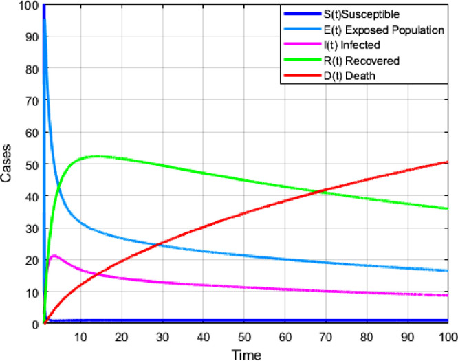
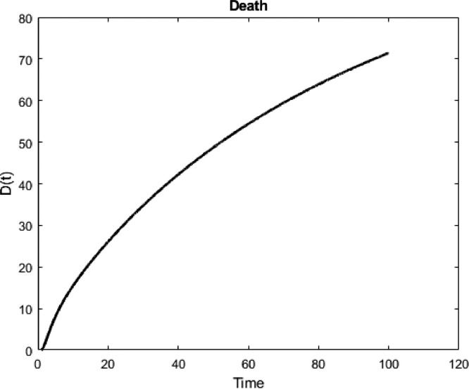
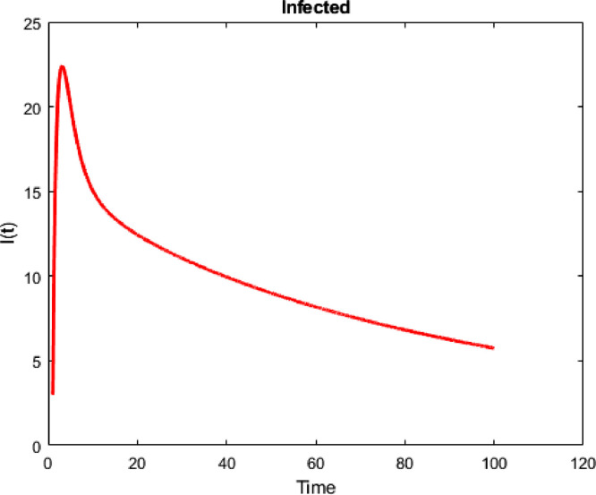
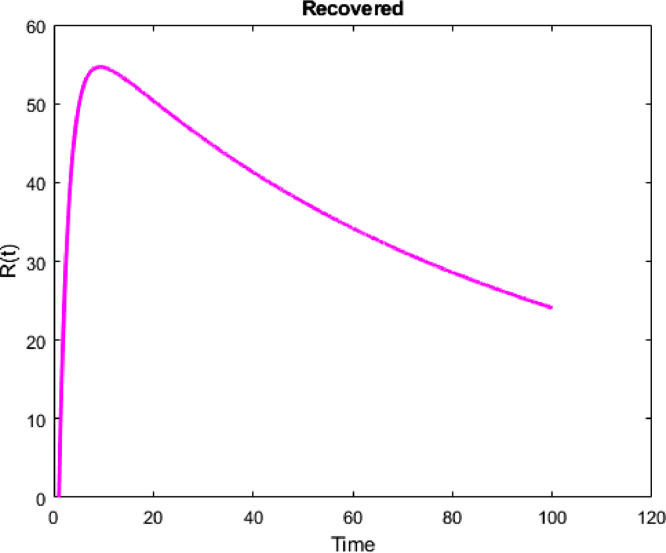
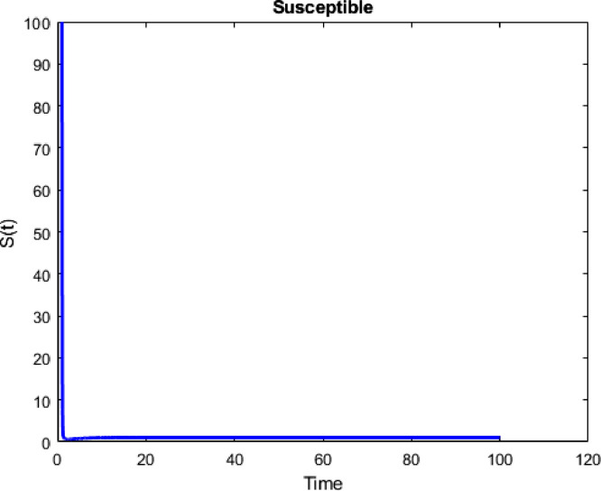
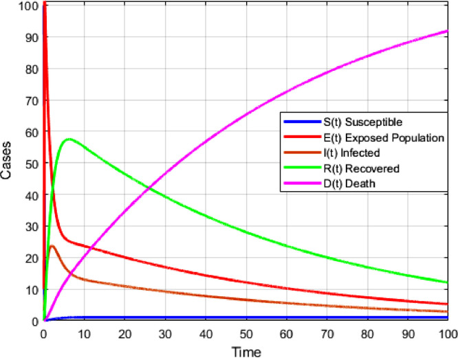
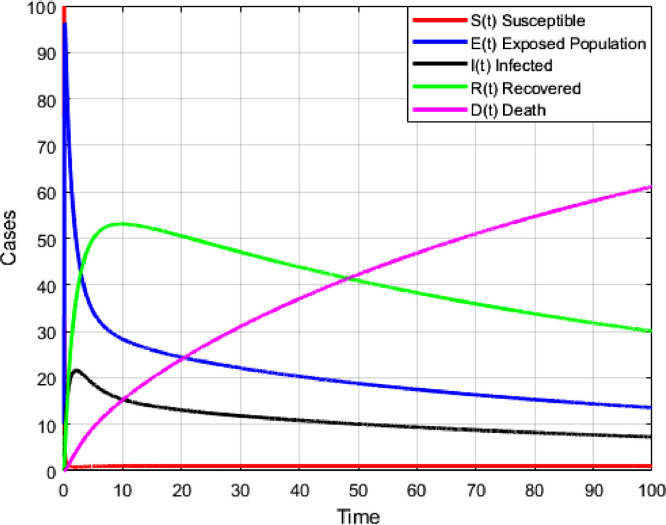
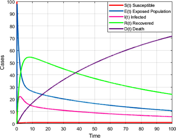
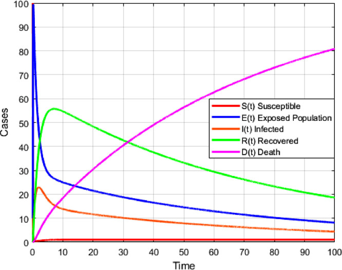
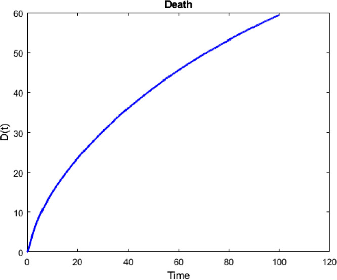
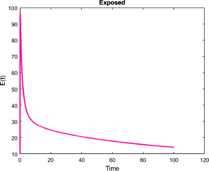
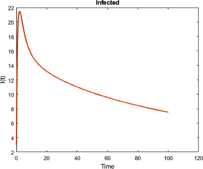
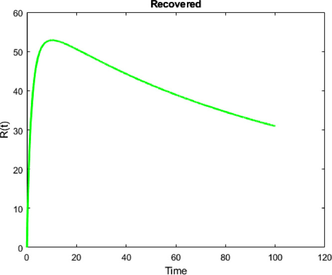
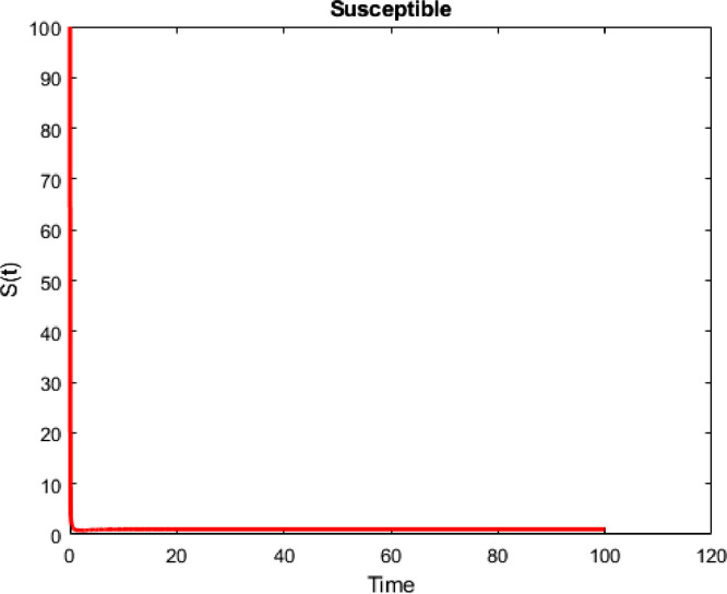
In this section, using the obtained numerical solutions, numerical simulations are performed for different values of fractional orders. The numerical simulation are thus depicted in Fig. 1, Fig. 2, Fig. 3, Fig. 4, Fig. 5, Fig. 6, Fig. 7, Fig. 8, Fig. 9, Fig. 10, Fig. 11, Fig. 12, Fig. 13, Fig. 14, Fig. 15, Fig. 16, Fig. 17 . Here the value we take is $\Lambda =0,{\alpha }_e=0.3,{\alpha }_i=0.4,r=0.23,k=0.3,\phi =0.25,\mu =0.12,\beta =0.45$ also we the initial condition value are $S\left(0\right)=100,E\left(0\right)=10,I\left(0\right)=3,R\left(0\right)=0,D\left(0\right)=0.$

Fig. 1.

Numerical Simulation for AB Derivative for α=0.79.

Fig. 2.

Numerical Simulation for AB Derivative for α=0.88.

Fig. 3.

Numerical Simulation for AB Derivative for α=0.91.

Fig. 4.

Numerical simulation for AB derivative of death class for the value of $\alpha =0.91$.

Fig. 5.

Numerical simulation for AB derivative of expressed population class for the value of $\alpha =0.91$.

Fig. 6.

Numerical simulation for AB derivative of Infected class for the value of $\alpha =0.91$.

Fig. 7.

Numerical simulation for AB derivative of recovered class for the value of $\alpha =0.91$.

Fig. 8.

Numerical simulation for AB derivative of susceptible class for the value of $\alpha =0.91$.

Fig. 9.

Numerical Simulation for AB Derivative for α=1.

Fig. 10.

Numerical Simulation for AB Derivative for α=0.85.

Fig. 11.

Numerical Simulation for AB Derivative for α=0.89.

Fig. 12.

Numerical Simulation for AB Derivative for α=0.94.

Fig. 13.

Numerical simulation for CF derivative for the death class for the value of $\alpha =0.85$.

Fig. 14.

Numerical simulation for CF derivative for the exposed class for the value of $\alpha =0.85$.

Fig. 15.

Numerical simulation for CF derivative for the infected class for the value of $\alpha =0.85$.

Fig. 16.

Numerical simulation for CF derivative for the recovered class for the value of $\alpha =0.85$.

Fig. 17.

Numerical simulation for CF derivative for the susceptible class for the value of $\alpha =0.85$.

11. Conclusion

To understand the propagation of covid-19 virus among humans, mathematician rely on the concept of differentiation and integration to construct linear and nonlinear ordinary or partial differential equations that could be used to depict not accurately but approximately the spread of the virus within a given population. They divide the total population in several sub-classes starting with susceptible, infected and deaths classes, these number are functions of time and space. The solution of these equations give human an indication on how severe the spread can be and what parameter is needed to control the spread. Thus in this paper a relatively simple and new mathematical model of covid-19 spread was suggested and analyzed. The model was further extended to capture more non-localities, the modified and the extended models were solved numerically using a recent developed numerical scheme based on the Newton polynomial interpolation, and finally numerical simulations are depicted for different values of fractional orders.

CRediT authorship contribution statement

Zizhen Zhang: Conceptualization, Data curation, Formal analysis, Funding acquisition, Investigation, Methodology, Project administration, Resources, Software, Supervision, Validation, Visualization, Writing - original draft, Writing - review & editing.

Declaration of Competing Interest

The authors declare that they do not have any financial or non- financial conflict of interests.

References

- 1.Atangana A., Dumitru B. New fractional derivatives with nonlocal and non-singular kernel: theory and application to heat transfer model. Therm Sci. 2016;18 doi: 10.2298/TSCI160111018A. [DOI] [Google Scholar]
- 2.Atangana A. The spread of COVID-19 with new fractal-fractional operators: can the lockdown save mankind before vaccination? Chaos Soliton Fract. 2020;136:109860. doi: 10.1016/j.chaos.2020.109860. [DOI] [PMC free article] [PubMed] [Google Scholar]
- 3.Atangana A., Araz S.I. New numerical method for ordinary differential equations: newton polynomial. J Comput Appl Math. 2020;372:112622. [Google Scholar]
- 4.Atangana A., Jain S. The role of power decay, exponential decay and mittag- leffler functions waiting time distributions: application of cancer spread. Physica A. 2019;33(512):330–351. doi: 10.1016/j.physa.2018.08. [DOI] [Google Scholar]
- 5.Chen W., Zhang X.D., Korosak D. Investigation on fractional and fractal derivative relaxation-oscillation models. Int J Nonlin Sci Num. 2010;11(2):3–9. [Google Scholar]
- 6.Caputo M., Fabrizio M. A new definition of fractional derivative without singular kernel. Prog Fract Differ Appl. 2015;1:73–85. [Google Scholar]
- 7.Jain S. Numerical analysis for the fractional diffusion and fractional Buckmaster’s equation by two step Adam- Bashforth method. Eur Phys J Plus. 2018;133:19. doi: 10.1140/epjp/i2018-11854-x. [DOI] [Google Scholar]
- 8.Khan M.A., Atangana A. Modeling the dynamics of novel coron- avirus (2019-ncov) with fractional derivative. Alexandria Eng J. 2020 doi: 10.1016/j.aej.2020.02.03. [DOI] [Google Scholar]
- 9.Diekmann O., Heesterbeek J.A.P., Metz J.A.J. On the definition and the computation of the basic reproduction ratio r 0 in models for infectious diseases in heterogeneous populations. J Math Biol. 1990;28:365–382. doi: 10.1007/BF00178324. [DOI] [PubMed] [Google Scholar]
- 10.Driessche P., Watmough J. Reproduction numbers and sub-threshold endemic equilibria for compartmental models of disease transmission. Math Biosci. 2002;180(1):29–48. doi: 10.1016/s0025-5564(02)00108-6. [DOI] [PubMed] [Google Scholar]
- 11.Chen Y., Cheng J., Jiang Y., Liu K. A time delay dynamic system with external source for the local outbreak of 2019-ncov. Appl Anal. 2020:1–12. [Google Scholar]