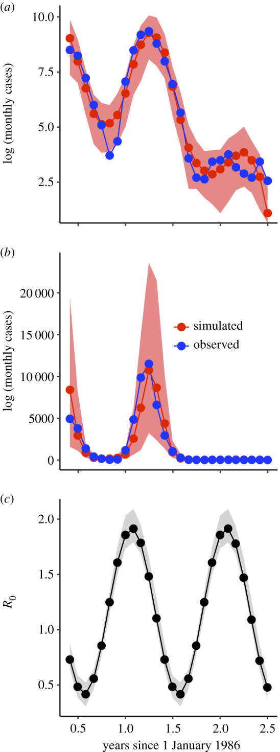
Figure 4.

(a,b) Comparison of simulated values with the fitted model and observed data on a log (a) and regular (b) scale. Observed monthly cases from April 1986 to June 1988 are shown in blue. Median values from 100 simulations with the maximum-likelihood parameter combination are shown in red. The shaded red region denotes the 2.5% and 97.5%th quantile boundaries from those simulations. (c) Estimates for R0(t). The black line denotes the trajectory of R0(t) for the maximum-likelihood estimate (MLE). The shaded grey region represents the 2.5% and 97.5%th quantile boundaries for trajectories from all parameter combinations within 2 log likelihood units of the MLE. Each parameter combination has only one seasonal trajectory for R0(t) because R0(t) is a deterministic quantity. R0(t) for all parameter estimates ranges from 1.79–2.09 in the on-season to 0.31–0.52 in the off-season.
