Figure 5:

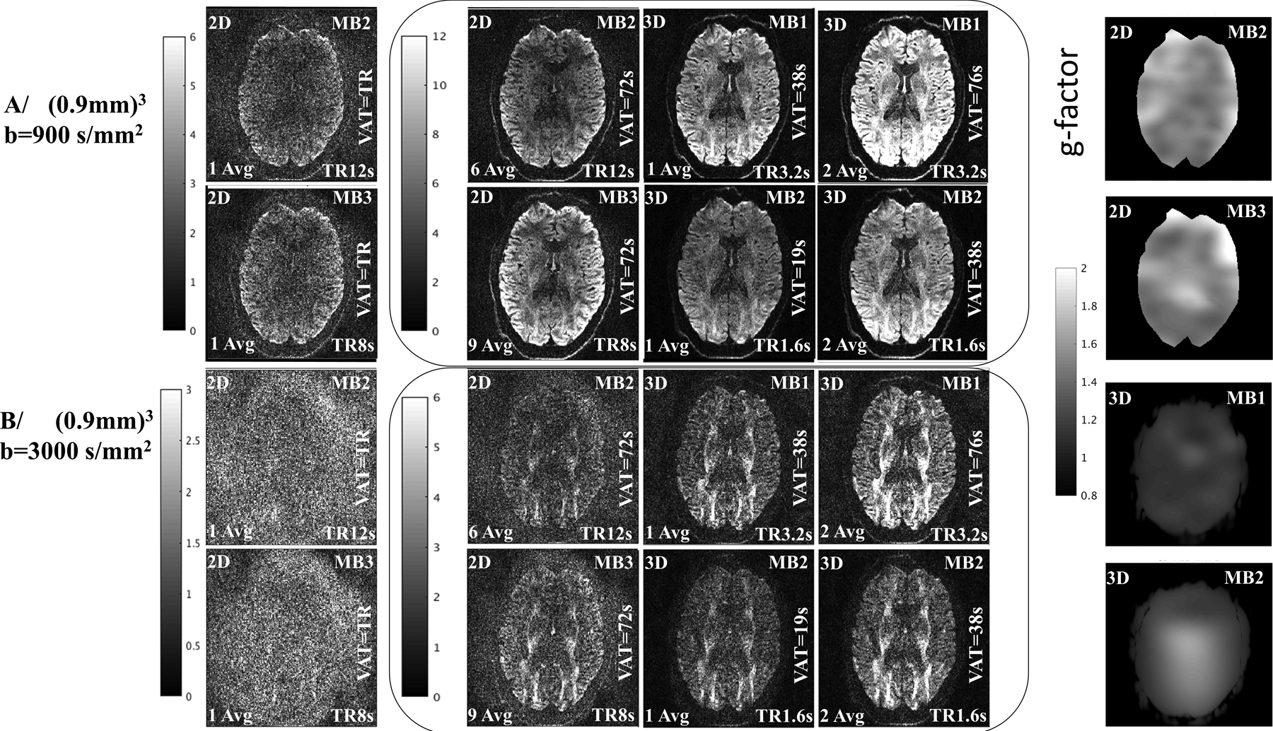
Comparison of the SNR in 2D and 3D acquisition for b=900 and 3000 s/mm² at (0.9mm)³ isotropic resolution. Column one in A/ and B/ are single average images obtained with 2D acquisitions using MB=2 (total acceleration 4) and MB=3 (total acceleration 6) respectively. The left column in the center figures in A/ and B/ are images obtained with the 2D acquisitions for VAT=72s obtained with averaging of complex valued signals. The center column in the center figures are images obtained with single averaged 3D acquisitions using MB=1(total acceleration 2, and VAT=38s) and MB=2(total acceleration 4 and VAT=19s) respectively. The right column in the center figures are images obtained with averaged 3D acquisitions using MB=1(total acceleration 2, and VAT=76s) and MB=2(total acceleration 4 and VAT=38s) respectively. The right column are images of g-factor maps for the corresponding slices obtained with the analytic g-factor method(61)