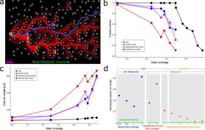
Figure 2. Ant vs simulation performances.
(a) Heat map of trajectories of 200 simulation iterations over an example maze (brighter colors signify more visits, cubes are drawn in white). Actual ant trajectory for this maze is overlaid in blue. Initial location for all trajectories is marked by a green cogwheel. (b) Probabilities to solve the maze as a function of mean coverage, for ants (blue), pinball model (red), and extended pinball model (magenta) simulations. The percent of solvable mazes is depicted in black (up to 0.55 coverage - experimental mazes, 0.55 coverage and above - computer generated mazes). Sample sizes (from small coverage to large): Ants - 15,57,19,19,28,30, Pinball Model - 200 iterations each over 10,14,10,8,15,11 distinct mazes, Extended Pinball Model - 500 iterations each over 10,14,10,8,15,11 distinct mazes. Existence of Solution - (experimental - up to 0.55 coverage): 10, 14, 10, 8, 15, 11 (generated- 0.55 coverage and beyond): 100 for each coverage. (c) Comparison of average total arc length of ants’ and different types of simulations’ trajectories (color scheme as in (b)). The geodesic shortest path traversing the maze is shown in black. We take into account the different success rates of the simulation and ants as shown in panel (b) by adding a penalty to each iteration/experiment which was not successful. The added penalty equals average speed multiplied by the time stuck before termination of experiment/iteration. Error margins in (b,c) are standard errors of the mean. Wherever no error is visible, the error is small enough to fit within the filled circle marker. Sample sizes (from small coverage to large): Ants - 31,10,14,10,8,15,11, Simulations - as in (b) except the first point is 200/500 iterations in the no cubes case, Shortest Path - 10,14,10,8,15,11, first point is simply the width of the board. (d) The performance of different simulated models normalized by empirical ant performance (marked by horizontal green line). We use a single inverse measure for the performance of the simulations, , where is the solution arc length (calculated as in panel (c)) averaged over all cube densities. Models are categorized by their locality and responsiveness, and separated into three differently colored x-axes; each corresponding to a different kind of simulation, wherein the numeric value is the main parameter we change in that simulation. Local non-responsive models are versions of the pinball model where noise levels were varied (Blue dots over blue axis, a noise value of 1 is the fitted value in original model. Appendix 2.1 and Appendix 2—figure 1). Local responsive models are versions of the pinball model in which noise is temporarily altered in response to the load being stuck in a trap (Red dots over red axis, Appendix 2.3 and Appendix 2—figure 3) or a new random bias direction is temporarily selected (Magenta dot over orange axis, Appendix 2.2 and Appendix 2—figure 2). The non-local responsive models are versions of the extended pinball model with different sensing radii (Orange dots over orange axis, Materials and methods, Appendix 2.4, Appendix 2—figure 4). For a full version of this panel with three additional simulations with considerably inferior performance, see Appendix 2—figure 5.

