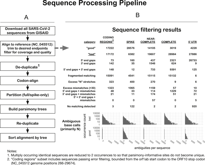
Figure S1.
Schematic of the SARS-CoV-2 Outbreak Sequence Processing Pipeline, Related to Figure 1
The intent of these procedures is to generate, for each of several regions, a set of contiguous codon-aligned sequences, complete in that region, without extensive uncalled bases, large gaps, or regions that are unalignable or highly divergent, in reasonable running time for n > 30,000 ∼30kb viral genomes. This allows daily processing of GISAID data to enable us to track mutations. This process provides the foundational data to enable the generation of Figures 1, 2, 3, and 7.
A. Processing procedures:
1. Download all SARS-CoV-2 sequences from GISAID.org (34,607 as of 2020-05-29). The downloaded sequences are stored in compressed form (via bzip2: https://sourceware.org/git/bzip2.git).
2. Align sequences to the SARS-CoV-2 reference sequence (NC_045512), trim to desired endpoints, and filter for coverage and quality. These steps are incorporated in a single Perl script, ‘align_to_ref.pl’, briefly summarized here: sequences are compressed for identity, then mapped against the given reference sequence using ‘nucmer’ from the ‘MUMmer’ package (Kurtz et al., 2004). The nucmer ‘delta’ file contains locations of matching regions and is parsed and used to, first, partition the sequences into “good” and “bad” subsets, and then to generate alignments from the “good” sequences.
B. Categories of sequences included and excluded from our automated alignments. A series of criteria is used successively to exclude sequences with large internal gaps, excessive five- and three-prime gaps, large numbers of mismatches or ambiguities (> 30) overall, or regions with a high concentration of mismatches or ambiguities (> 10 in any 100 nt subsequence): the counts of these categories of “bad” sequence are shown, for different regional genome alignments.
We then create the following different regional subalignments: CODING-REGIONS2 (“FULL,” from the 5′-most start-codon (orf1ab) to the 3′-most stop-codon (ORF10), NC_045512 bases 266-29,674; SPIKE, the complete surface glycoprotein coding region, bases 21,563-25,384; NEAR-COMPLETE (“NEARCOMP,” the most-commonly-sequenced region of the genome, bases 55-29,836; COMPLETE, matching the NC_045512 sequence from start up to the poly-A tail, bases 1-29,870; 5′ UTR, the five-prime untranslated region, bases 1-265 only. Generally speaking, the smaller the region, the more sequences are included.
Sequences are trimmed to the extent of the reference (with minimum allowed gaps at 5′ and 3′ ends), following which the pairwise alignments are generated from the matching regions, and a multiple sequence alignment is constructed from the pairwise alignments.
3. De-duplicate1. To reduce computational demands, sequences are compressed by identity following trimming to the desired region, by computing a hash value for each sequence (currently the SHA-1 message digest, 160 bits encoded as a 40-character hex string). To prevent the loss of parsimony-informative characters when they occur in identical strings, however, multiple sequences are reduced to a minimum of two occurrences.
4. Codon-align. Gaps are introduced into the entire compressed alignment so that the alignment column containing the last base of each codon has a number divisible by three; this simplifies processing of translations. Code for this procedure is derived from the GeneCutter tool from the LANL HIV database (https://www.hiv.lanl.gov/content/sequence/GENE_CUTTER/cutter.html).
5. Partition (full/spike-only). For subalignments that encompass the spike protein and substantial additional sequence, the spike region is extracted separately, to allow matched comparisons.
6. Build parsimony trees. A brief parsimony search (parsimony ratchet, with 5 replicates) is performed with ‘oblong’ (Goloboff, 2014) This is intended as an efficient clustering procedure rather than an explicit attempt to achieve an accurate phylogenetic reconstruction, but it appears to yield reasonable results in this situation of a very large number of sequences with a very small number of changes, where more complex models may be subject to overfitting. When multiple most-parsimonious trees are found, only the shortest of these (under a p-distance criterion) is retained. Distance scoring is performed with PAUP∗ (Swofford, 2003).
7. Re-duplicate (expand, i.e., uncompress). The original sequence names and occurrence counts are restored to FastA format files and the appropriate leaf taxa added to the parsimony trees.
8. Sort alignment by tree. Sequences in the FastA files are sorted by the expanded tree, allowing patterns of mutation to be discerned by inspection.
9. Mutations of interest can be readily tracked on the trees to resolve whether they are identified in predominantly in single clades or distributed throughout the tree and likely to be recurring (e.g., Figure 7 (sites of interest with low frequency amino acid substitutions) and Figure S6 (Site 614)).

