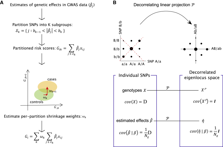
Figure 1.

Overview of Non-Parametric Shrinkage (NPS)

(A) For unlinked markers, NPS partitions SNPs into K subgroups splitting the GWAS effect sizes (${\hat{\beta }}_j$) at cut-offs of $b_0,b_1,\dots ,b_K$. Partitioned risk scores $G_{ik}$ are calculated for each partition $k$ and individual $i$ using an independent genotype-level training cohort. The per-partition shrinkage weights ${\omega }_k$ are determined by the separation of $G_{ik}$ between training case subjects and control subjects. Estimating the per-partition shrinkage weights is a far easier problem than estimating per-SNP effects. The training sample size is small but still larger than the number of partitions, whereas for per-SNP effects, the GWAS sample size is considerably smaller than the number of markers in the genome. This procedure “shrinks” the estimated effect sizes not relying on any specific assumption about the distribution of true effect sizes.

(B) For markers in LD, genotypes and estimated effects are decorrelated first by a linear projection $\mathcal{P}$ in non-overlapping windows of ∼2.5 Mb in length, and then NPS is applied to the data. The size of black dots indicates genotype frequencies in population. Before projection, genotypes at SNP 1 and 2 are correlated due to LD ($\mathbf{D}$), and thus sampling errors of estimated effects (${\hat{\beta }}_j|{\beta }_j$) are also correlated between adjacent SNPs. The projection $\mathcal{P}$ neutralizes both correlation structures. The axes of projection are marked by red dashed lines. ${\beta }_j$ denotes the true genetic effect at SNP $j$. $N_g$ is the sample size of GWAS cohort.