An analysis of COVID-19 spread based on fractal interpolation and fractal dimension

Abstract

The present paper proposes a reconstruction of the epidemic curves from the fractal interpolation point of view. Looking at the epidemic curves as fractal structures might be an efficient way to retrieve missing pieces of information due to insufficient testing and predict the evolution of the disease. A fractal approach of the epidemic curve can contribute to the assessment and modeling of other epidemics. On the other hand, we have considered the spread of the epidemic in countries like Romania, Italy, Spain, and Germany and analyzed the spread of the disease in those countries based on their fractal dimension.

1. Introduction

In the last 100 years, there have been many pandemics from the Spanish Flu (1918–1919), Asian Flu (1957), Hong Kong Flu (1968), etc. (see [27]) Most of them have occurred due to different influenza virus serotypes. Coronaviruses are known for being pathogens that affect mostly the animals. Recently, an increasing number of tests and researches have been performed to identify the outcome of human infection with coronavirus serotypes. Coronaviruses are endemic in some areas, generating mild diseases, but in the last years, some strains have emerged leading to severe-lethal diseases like Severe Acute Respiratory Syndrome coronavirus (SARS-CoV-1) 2003 and Middle East Respiratory Syndrome coronavirus (MERS-CoV) 2012 (see [28]).

At the end of December 2019, China has reported to the World Health Organization (WHO) an outbreak of a severe respiratory infectious disease in Wuhan. WHO has announced, on January $7^{\text{th}},$ that the genome of the viral pathogen has been identified as a new coronavirus (nCov/ novel coronavirus/ COVID-19/ SARS-CoV-2). During January and the first week of February SARS-CoV-2 has been developing as an epidemic in the region, affecting mostly China, but also Japan, Thailand, Vietnam, etc. Few cases have been reported in the same period also in some other parts of the globe as, for example, France, Germany, Spain, and Italy in Europe, the United States of America, Australia. From that moment, in just one month, the epidemic has been reclassified as a pandemic (see [28]). Now it has affected all the countries of the world in a different proportion.

The source of the new coronavirus is still unidentified, but Zhou et al. (see [31]) have observed that the genome of the SARS-CoV-2 is 96% similar to RaTG13, coronavirus sampled from Rhinolophus affinis bat. Zhang et al. (see [30]) have suggested that some coronaviruses identified from pangolin species are similar in the receptor-binding domain with SARS-CoV-2. Reviewing all the data, Andersen et al. (see [2]) have concluded that the natural selection of the virus could have happened in animals, before zoonotic transmission, or in humans, after zoonotic transmission.

In the battle with this viral infectious disease, humanity has had to find some basic epidemiological data about the pathogen, such as the way of transmission, reproduction number, incubation period, the population mostly affected, etc. Out of those data, we should mention the reproduction number (R ₀) which means how many new cases will be generated by an infected person among healthy people. A high R ₀ suggests that the virus is still spreading, while a low R ₀ indicates that the epidemic may extinct (see [11]). The scientists have used the data gathered recently and have tried to model the epidemic so that they can predict the evolution of the disease (see [16], [18]). Also, by using these models, the specialists may recommend a set of rules to reduce the impact of the virus within the population. Active surveillance of positive cases, and contact finding is one of the best ways to control the pandemic (see [8]). Not only surveillance but also social distancing has shown great results in flattening the curve. It is utmost important that those two strategies are combined for the best impact (see [23]), as Ghosh et al. (see [14]) have observed through a Stochastic Computational Simulation Model, the combination of social distancing, increase detection rates and improvement in hospital bed numbers can reduce the impact of the Covid-19 in the population. To evaluate if those measures have helped and have reduced the reproduction rate, we may compare the epidemic curves generated for prediction to the real ones, obtained from WHO or from each country’s public health department.

The epidemic curves are represented on an xOy graphic, where Ox axis corresponds to Time, while the Oy axis is the number of people infected. There are three types of epidemic curves i.e. point source outbreak, common source outbreak, propagated outbreak. The last one is characteristic for SARS-CoV-2, as the pathogen is spreading from person to person. The epidemic curve can be projected during the outbreak using stochastic methods to predict the evolution of the epidemic or can be plotted after the end of the epidemic to understand the dynamic of the disease better. The stochastic method is used more and more for predicting the evolution of the outbreak. The dynamic modeling, in which data is obtained from heterogeneous sources, is constantly improving and is going to be done through fully stochastic transmission models (see [9]). The big challenge is to obtain a method to predict the development of an infectious outbreak when data is not always complete and it is highly noisy (see [12]). We have observed that the noisy information can present a pattern, resembling a fractal. Through this article we try to evaluate the epidemic curves using a fractal point of view, searching for new information that can be useful for comparing different outbreaks or predictions. The pandemic is still active so that the final epidemic curves may be different in the end, as rectifications are usually done some months after the outbreak‘s extinction.

Analyzing the expansion of the Covid-19 disease from the fractal analysis point of view might help in getting a better insight into the complexity of the disease and the way it differed from other epidemics that the world has encountered in the past. Although there have been articles that model how the epidemic has spread (see [24], [19], [3]), or analyze and predict (see [13], [1], [17]) the epidemic, the current paper presents a fractal perspective, which has not been considered yet, which brings interesting outcomes. Considering the spread of the epidemic as a fractal structure might benefit the medical community in a better understanding not only of the present medical crisis generated by Covid-19 but it can also be a useful tool in further assessing other epidemics and their evolution.

2. Materials and methods

All the data considered for daily cases and daily tests is gathered from ourworldindata.org (see [33]).

One of the main classes of fractals consists of the graphs of continuous functions which are not derivable at any point. These types of functions have a very jagged outlook while keeping a great deal of similarity.

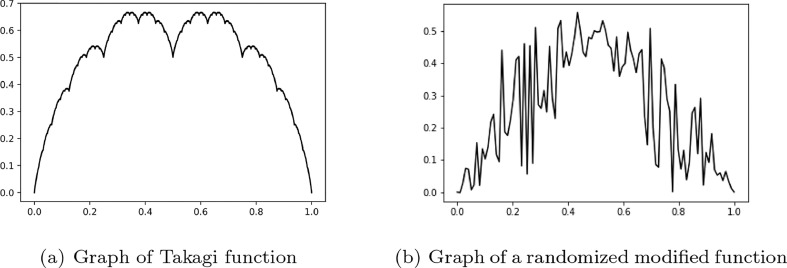
One example of such fractal is provided by the Blancmange curve (see [37]). This curve was described by Teiji Takagi in 1901 and it is also known as the Takagi curve, after him. We can construct the curve with the aid of the function $\theta :\mathbb{R}\to \mathbb{R}$ which measures the distance from every point x to its closest integer: $\theta \left(x\right)=dist(x,\mathbb{Z})$.

We compute the graph of an approximation of the Takagi function for an n great enough in Fig. 1 (a). This graph is a classical example of a fractal.

Fig. 1.

Examples of fractals.

Modifying the form of this function as

$${\tau }^{*}\left(x\right)=\sum _{i=0}^n\frac{1}{c^i}\theta \left(2^{i}x\right),\text{for}\text{every}x\in [0,1],$$

with c varying between $(-2,2)$ we obtain new functions. The graph in Fig. 1(b) is obtained for computing the function τ*(x) for 100 linearly spaced points in the interval [0,1], with c randomly chosen in $(-2,2)$ at each iteration. The Python code used is listed below

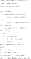
The outlook of the newly obtained curve is rather jagged and although it possesses a significantly less amount of similarity, it still has a fractal structure.

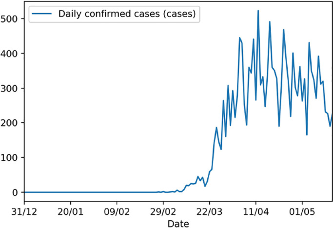
Taking a look at the data of the daily new cases of Covid-19 for various countries, the graph tends to have a rather jagged and irregular form. The daily new cases recorded in Romania are represented in Fig. 2 .

Fig. 2.

Daily cases of Covid-19 reported in Romania.

The graph in Fig. 1(b) of a classical fractal can be compared to the graph of the daily number of cases recorded in Romania in Fig. 2. The case is similar for most of the countries where Covid-19 cases were recorded.

Taking into account the noticeable similarity between the fractal in Fig. 1(b) and the daily new cases recorded for Romania in Fig. 2, considering the daily new Covid-19 cases recorded for each country as a fractal is well justified.

Fractal interpolation of data requires a continuous function that is to cross through each of the points on the dataset. The technique of fractal interpolation has been a subject of interest for many papers. A survey on fractal interpolation, containing a significant amount of results in the field of fractal interpolation, can be consulted in Fractal interpolation functions: a short survey (see [25]). The mathematical foundation of fractal interpolation has been laid in articles and books such as [21], [5], [6], [7]. Fractal interpolation has applications in a variety of areas (see [22]), from curve fitting (see [20]), to reconstructing satellite images (see [10]), and many others.

We have a set of points which have on the first component, x_i, the index of the date of the outbreak, where x ₀ is 0 and represents the first day of the outbreak and x_n is N and corresponds to the last entry in each of the datasets considered, and on the second component, y_i, represented by the corresponding number of cases recorded in the i-th day of the outbreak.

In order to interpolate the data, we need to build the fractal interpolation function. The program used to interpolate the data is an implementation in Python of the algorithm presented by Barnsley in Fractals everywhere, Chapter IV (see [4]).

We consider the following equations

$$\begin{array}{c}{a}_n=\frac{x_n-x_{n-1}}{x_N-x_0}\\ b_n=\frac{x_N{x}_{n-1}-x_0{x}_n}{x_N-x_0}\\ c_n=\frac{y_n-y_{n-1}}{x_N-x_0}-d_n\frac{y_N-y_0}{x_N-x_0}\\ e_n=\frac{x_n{y}_{n-1}-x_o{y}_n}{x_N-x_0}-d_n\frac{x_N{y}_0-x_o{y}_n}{x_N-x_0},\end{array}$$ (1)

where d_n is random, but fixed in (0,1).

To interpolate the data set, we based our program mainly on the numpy package which allows an easy way to work with arrays. Each of the equations from (1) were built separately as an array (A, B, C, E) which stores all N values. We considered O an array of zeros of length $N-1$ and D an array of the same dimensions filled with 0.1. The individual arrays were transformed in column arrays and concatenated in the order A, O, B, C, D, E. Based on this matrix we constructed the interpolation function by implementing the following formula:

$$\begin{array}{c}\hfill f\left(\begin{array}{c}{\displaystyle x}\hfill \\ {\displaystyle y}\hfill \end{array}\right)=\left(\begin{array}{cc}{\displaystyle a_k}\hfill & {\displaystyle 0}\hfill \\ {\displaystyle c_k}\hfill & {\displaystyle d_k}\hfill \end{array}\right)+\left(\begin{array}{c}{\displaystyle b_k}\hfill \\ {\displaystyle e_k}\hfill \end{array}\right).\end{array}$$ (2)

The box-counting dimension, or Minkowski dimension, or Minkowski-Bouligand dimension, is a way of measuring the fractal dimension of an object. Briefly, it is computed by counting how many boxes of a certain length are required to cover the object.

Given a subset S of ${\mathbb{R}}^2,$ the box-counting dimension of S is given by the formula

$$d_{box-counting}\left(X\right)=\frac{\ln \left(N\right(s\left)\right)}{\ln \left(\frac{1}{s}\right)}$$

where N(s) represents the number of sets of the form $[m_{1}s,(m_1+1)s]\times [m_{2}s,(m_2+1)s],$ where $m_1,m_2\in \mathbb{N}$ and s > 0, which intersect S.

For computing the box-counting dimension, we built a program in Python, based on the code in [29].

To determine how fractal the spread of Covid-19 is across the territory of a country, a map of the confirmed cases per region is needed. For Romania, using GeoGebra (see [15]), we built such a map of the number of cases for each region, based on the data available (see [32]).

For Italy, Germany, and Spain, we also considered maps, that we created in GeoGebra, of the number of cases per region based on data available at [34] and analyzed their fractal dimensions.

For the assessment of the degree of fractality based on this map, we used the box-counting dimension.

The main tool used in analyzing the data collected regarding Covid-19 and in computing all the graphics is Python programming language, more specifically, the pandas package.

3. Results

3.1. Fractal interpolation of daily cases data

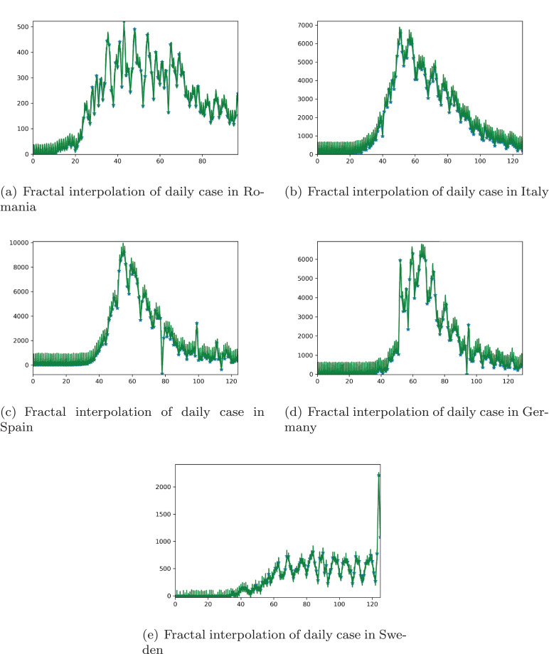
Analyzing the data of the daily cases reported for Romania, Italy, Spain, Germany, and Sweden, the irregularities are highly visible. Thus, the idea of choosing fractal interpolation of the data is significantly relevant.

The daily data of recorded cases are interpolated with the aid of a program in Python that interpolates the data according to Eqs. 1, where d_n is considered 0.1. The starting point x ₀ is 0 and corresponds to the day of the first recorded case of Covid-19 for the considered country. A more detailed description of the first confirmed case and the number of entries in the database can be visualized in Table 1 .

Table 1.

Data recorded per country.

Country	First case	Number of days since	Number of days
	confirmed	first confirmed case	with confirmed cases
Romania	Feb 27	98	95
Italy	Jan 31	127	106
Spain	Feb 1	125	103
Germany	Feb 1	126	110
Sweden	Jan 28	130	101

Thus, Fig. 3 depicts the interpolated data of the daily confirmed cases in the specified country.

Fig. 3.

Fractal interpolation of daily case per country.

Hence, the considered data interpolated as in Fig. 3 can be regarded as a fractal.

3.2. Fractal interpolation of daily testing data

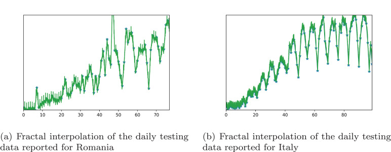
Since the significance of testing data for each day is indisputable in analyzing the complexity of the evolution of Covid-19, we collected the data for Romania and Italy - Germany, Spain, and Sweden did not give publicly the daily testing data - for comparison.

Hence, Fig. 4 depicts the result of the fractal interpolation of daily testing data recorded for Romania and Italy.

Fig. 4.

Fractal interpolation of daily tests per country.

3.3. Fractal dimension of covid-19

The map of reported cases in a country might give us an inside upon the manner Covid-19 disease has spread in that territory. The understanding of how complex the spreading of the virus within a country is can be a useful tool in further assessing not only how affected a certain area has been, but also how well the authorities responded to the crisis.

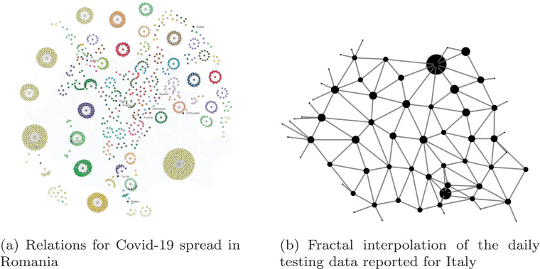
For the first analysis, let us consider the confirmed cases per each county in Romania. To assess the fractal dimension of Covid-19 in Romania, we marked the main border points which have functioned as the main vector origins for the viral dissemination over the country. Mapping the border crossing points which remained open and connecting the adjacent counties is highly relevant if we evaluate the relationship of the Covid-19 cases in Romania, in Fig. 5 (a)1 . The relationship of the confirmed Covid-19 cases in Romania clearly indicates the existence of interconnected clusters.

Fig. 5.

Map of Covid-19 cases in Romania counties.

Computing the fractal dimension on the map Fig. 5(b), we get a dimension of 1.4, which might give us an inside of the complexity of the spread of Covid-19 when compared to other countries.

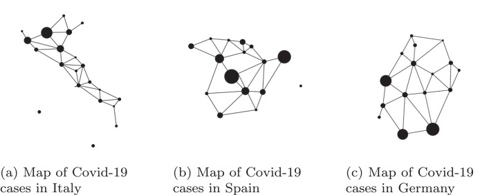
In order to make a comparison between the fractal dimension in different countries, we considered the maps of cases per region as per the situation on May ${}^{{21}^{\mathit{st}}}$ 2020, for Italy, Spain and Germany, and computed their fractal dimension. The results of the computed dimensions for the maps in Fig. 6 are noted in Table 2 .

Fig. 6.

Map of Covid-19 cases in specified country.

Table 2.

Data recorded per country.

Country	Fractal dimension computed
Italy	1.2193
Spain	1.2865
Germany	1.3222

4. Discussions

The relevance of approaching the epidemiological curve as a fractal has advantages from two points of view.

First of all, since the daily increase in the number of cases is rather irregular and hard to predict, the perspective of it as being a fractal might open a new way of predicting the evolution of the epidemic. Since the graph is fractal, besides being jagged and broken, it possesses some kind of fractal architecture that is prone to self-similarity. This similarity is a key element in assessing the current condition and predicting the next modifications in the epidemiological curves.

On the other hand, regarding the epidemiological curve as a fractal and computing it as the result of fractal interpolation might be an effective means in reconstructing pieces of data that have not been recorded. In this respect, we need to underline that the number of cases recorded is highly dependent on the number of tests performed by each country on a certain day. Analyzing the data employing fractal interpolation we can cover some pieces of data that might be missing to get a better picture of the epidemic.

Computing the fractal dimension of the epidemic curves, one will obtain similar results because of the d_n parameter. Eventually, the fractal dimension of the epidemic curves, selected for this paper, will not reveal exactly the evolution of the epidemic in Italy, Spain, Germany, Romania, and Sweden. Even though we have not obtained relevant information by computing the fractal dimension, we have demonstrated that the epidemic curves resemble a fractal structure. It has been observed that fractal statistic study may reveal further information (see [26]), but this has not been the subject of this paper.

4.1. An outlook of covid-19 in the world

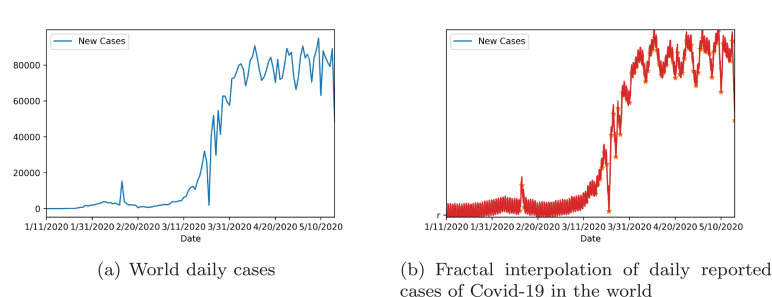
Since Covid-19 has become a pandemic, an outlook upon the evolution of the disease for the entire world is necessary. The daily cases recorded globally since the first case was announced are graphed in Fig. 7 (a).

Fig. 7.

Fractal interpolation of daily tests per country.

Since globally testing has been difficult in many areas and confirmed cases are inconsistent in some places, reconstructing the data through fractal interpolation might give a better insight into how the cases have evolved. Moreover, fractal interpolation of the daily cases can complete some missing pieces of information for certain days.

Thus, Fig. 7(b) shows the result of the fractal interpolation of data for daily confirmed cases globally.

4.2. Fractal dimension

In terms of the fractal dimension of the Covid-19 disease spread on the territory of a country, two points of view are to be analyzed.

Firstly, we can consider a map, as in Fig. 5(b), where we have taken into consideration the connections between certain clusters of infection. Computing the fractal dimension, in this case, gives us an inside upon the spread of the disease in Romania based on the variety of ways the virus has traveled. The computed dimension of 1.4 signals that the complexity of the spread of the disease is rather high and it is influenced by the existing connections between infection clusters.

On the other hand, computing the fractal dimension based on the map of cases available at [34], we can get an inside of how affected a country has been.

From an epidemic point of view, observing the fractal dimension of each map we may comment on some epidemic characteristics of this disease. The crucial information about the SARS-CoV-2 that can be obtained from the fractal dimension of the map is how the virus has spread inside a country. While Italy has had an important cluster in the North, Lombardy region with almost 40% of the positive cases, with less important clusters scattered in each region (see [35]), the fractal dimension computed has been 1.21. In Spain, two main clusters, Madrid and Cataluna, had more than 52% of the positive cases (see [36]). The other 48% have been located in small clusters. The fractal dimension of Spain is 1.28 which suggests a higher complexity of case distribution. Germany, even though not so affected by this novel coronavirus, has a higher value for the fractal dimension, 1.32, because there have been 3 main clusters and other medium and small (see [34]). It is important to mention that from the graphs in Fig. 6 we may observe the distribution but not how many people have been infected. The complexity of distribution can be used to backtrack the source of the epidemic and to assess whether the lockdown measures have been useful and have limited the spreading.

5. Conclusion

To sum up, fractals can be used to assess an epidemic outbreak. As we have observed, the epidemic curves can be recreated using fractal methods, more precisely, fractal interpolation techniques. Even though the idea of using fractals to observe an epidemic is not new, recreating the epidemic curve employing fractal interpolation has not yet been applied. Moreover, we have tried to see whether the complexity of an outbreak can be quantified by using the fractal dimension. By comparing the regions in every state, we may observe whether the measures to reduce the spreading had been useful or not. It is important to mention that a final conclusion of this idea can be drawn only after the end of the epidemic, after the last rectifications. At this moment we can just observe if the disease has dispersed uniform inside a country or it has been located mostly in one source.

This paper has tried to model the SARS-CoV-2 pandemic as a fractal structure. We have used retrospective data to create those models. The next step should be the generation of a fractal prediction method that takes into account the variables of this epidemic.

CRediT authorship contribution statement

Cristina-Maria Păcurar: Conceptualization, Formal analysis, Funding acquisition, Data curation, Writing - review & editing, Writing - original draft, Visualization. Bogdan-Radu Necula: Writing - original draft, Formal analysis, Funding acquisition, Data curation, Writing - review & editing, Visualization.

Declaration of Competing Interest

The authors declare that they have no known competing financial interests or personal relationships that could have appeared to influence the work reported in this paper.

References

- 1.Anastassopoulou C., Russo L., Tsakris A., Siettos C. Data-based analysis, modelling and forecasting of the COVID-19 outbreak. PLoS ONE. 2020;15(3):e0230405. doi: 10.1371/journal.pone.0230405. [DOI] [PMC free article] [PubMed] [Google Scholar]
- 2.Andersen K.G., Rambaut A., Lipkin W.I., Holmes E.C., Garry R.F. The proximal origin of SARS-cov-2. Nature Medicine. 2020;26:450–452. doi: 10.1038/s41591-020-0820-9. [DOI] [PMC free article] [PubMed] [Google Scholar]; No. -, https://www.nature.com/articles/s41591-020-0820-9
- 3.Barmparis G.D., Tsironis G.P. Estimating the infection horizon of COVID-19 in eight countries with a data-driven approach. Chaos Solitons & Fractals. 2020:109842. doi: 10.1016/j.chaos.2020.109842. [DOI] [PMC free article] [PubMed] [Google Scholar]
- 4.Barnsley M. 3rd Edition. Dover Publications; 2012. Fractals everywhere. [Google Scholar]
- 5.Barnsley M.F. Fractal functions and interpolation. Constr Approx. 1986;2:303–329. doi: 10.1007/BF01893434. [DOI] [Google Scholar]
- 6.Barnsley M.F., Elton J., Hardin D., Massopust P.R. Hidden variable fractal interpolation functions. SIAM J Math Anal. 1989;20:1218–1242. [Google Scholar]
- 7.Barnsley M.F., Harrington A.N. The calculus of fractal interpolation functions. J Approx Theory. 1989;57:14–34. doi: 10.1016/0021-9045(89)90080-4. [DOI] [Google Scholar]
- 8.Bedford J., Enria D., Giesecke J., Heymann D.L. COVID-19: towards controlling of a pandemic. The Lancet. 2020;395(10229):1015–1018. doi: 10.1016/S0140-6736(20)30673-5. [DOI] [PMC free article] [PubMed] [Google Scholar]; Https://www.thelancet.com/journals/lancet/article/PIIS0140-6736(20)30673-5/fulltext.
- 9.Birrell P.J., Angelis D.D., Presanis A.M. Evidence synthesis for stochastic epidemic models. Stat Sci. 2018;33(1):34–43. doi: 10.1214/17-STS631. [DOI] [PMC free article] [PubMed] [Google Scholar]
- 10.Chen C.J., Cheng S.C., Huang Y.M. The reconstruction of satellite images based on fractal interpolation. Fractals. 2011;(19):347–354. doi: 10.1142/S0218348X11005385. [DOI] [Google Scholar]
- 11.Delamater P.L., Street E.J., Leslie T.F., Yang Y.T. Complexity of the basic reproduction number (r0) Emerg Infect Dis. 2019;25(1):1–4. doi: 10.3201/eid2501.171901. [DOI] [PMC free article] [PubMed] [Google Scholar]
- 12.Dureau J., Kalogeropoulos K., Baguelin M. Capturing the time-varying drivers of an epidemic using stochastic dynamical systems. Biostatistics. 2013;14(3):541–555. doi: 10.1093/biostatistics/kxs052. [DOI] [PubMed] [Google Scholar]
- 13.Fanelli D., Piazza F. Analysis and forecast of COVID-19 spreading in china, italy and france. Chaos, Solitons & Fractals. 2020;134:109761. doi: 10.1016/j.chaos.2020.109761. [DOI] [PMC free article] [PubMed] [Google Scholar]
- 14.P G., Basheer S., Paul S., Chakrabarti P., Sarkar J. Increased detection coupled with social distancing and health capacity planning reduce the burden of COVID-19 cases and fatalities: A proof of concept study using a stochastic computational simulation model. medRxiv. 2020 [Google Scholar]; Https://www.medrxiv.org/content/10.1101/2020.04.05.20054775v1
- 15.Hohenwarter M., Borcherds M., et al. Geogebra. 2018. 5.0.507.0, http://www.geogebra.org.
- 16.Kucharski A.J., Russell T.W., Diamond C., Liu Y. Early dynamics of transmission and control of COVID-19: a mathematical modelling study. Lancet Infect Dis. 2020;20(5):553–558. doi: 10.1016/S1473-3099(20)30144-4. [DOI] [PMC free article] [PubMed] [Google Scholar]
- 17.Libotte B.G., Lobato F., Gustavo M.P. Identification of an epidemiological model to simulate the COVID-19 epidemic using robust multi-objective optimization and stochastic fractal search. arXiv e-prints. 2020 doi: 10.1155/2020/9214159. [DOI] [PMC free article] [PubMed] [Google Scholar]; ArXiv:2006.00289, https://ui.adsabs.harvard.edu/abs/2020arXiv200600289B
- 18.Liu Y., Gayle A.A., Wilder-Smith A., Rocklöv J. The reproductive number of COVID-19 is higher compared to SARS coronavirus. J Travel Med. 2020;27(2) doi: 10.1093/jtm/taaa021. [DOI] [PMC free article] [PubMed] [Google Scholar]; P. taaa021
- 19.Mandal M., Jana S., Nandi S.K., Khatua A., Adak S., Kar T.K. A model based study on the dynamics of COVID-19: prediction and control. Chaos,Solitons & Fractals. 2020:109889. doi: 10.1016/j.chaos.2020.109889. [DOI] [PMC free article] [PubMed] [Google Scholar]
- 20.Manousopoulos P., Drakopoulos V., Theoharis T. In: Transactions on Computational Science I. Lecture Notes in Computer Science, vol 4750. Gavrilova M.L., Tan C.J.K., editors. Springer; Berlin, Heidelberg: 2008. Curve fitting by fractal interpolation. [Google Scholar]; DOI: 10.1007/978-3-540-79299-4_4
- 21.Massopust P.R. Academic Press; San Diego, CA, USA: 1994. Fractal functions, fractal surfaces and wavelets. [Google Scholar]
- 22.Massopoust P. Fractal functions and their applications. Chaos Solitons & Fractals. 1997;8:171–190. [Google Scholar]
- 23.Matrajt L., Leung T. Evaluating the effectiveness of social distancing interventions to delay or flatten the epidemic curve of coronavirus disease. Emerg Infect Dis. 2020 doi: 10.3201/eid2608.201093. [DOI] [PMC free article] [PubMed] [Google Scholar]; Aug. https://doi.org/10.3201/eid2608.201093
- 24.Ndaïrou F., Area I. Mathematical modeling of COVID-19 transmission dynamics with a case study of wuhan. Chaos, Solitons & Fractals. 2020;135:109846. doi: 10.1016/j.chaos.2020.109846. [DOI] [PMC free article] [PubMed] [Google Scholar]
- 25.Navascues M., Chand A., Veedu V., Sebastian M. Fractal interpolation functions: a short survey. Appl Math (Irvine) 2014;5:1834–1841. doi: 10.4236/am.2014.512176. [DOI] [Google Scholar]
- 26.Nygård J.F., Glattre E. Fractal analysis of time series in epidemiology: is there information hidden in the noise? Norsk Epidemiologi. 2003;13(2):303–308. doi: 10.5324/nje.v13i2.300. [DOI] [Google Scholar]
- 27.Potter C. A history of inluenza. J Appl Microbiol. 2001;91:572–579. doi: 10.1046/j.1365-2672.2001.01492.x. [DOI] [PubMed] [Google Scholar]; No. -
- 28.Raoult D., Zumla A., Locatelli F., Ippolito G., Kroemer G. Coronavirus infections: epidemiological, clinical and immunological features and hypotheses. Cell Stress. 2020;4(4):66–75. doi: 10.15698/cst2020.04.216. [DOI] [PMC free article] [PubMed] [Google Scholar]
- 29.Rougier N.P.. https://gist.github.com/rougier/e5eafc276a4e54f516ed5559df4242c0.js.
- 30.Zhang T., Wu Q., Zhang Z. Pangolin homology associated with 2019-ncov. bioRxiv. 2020 [Google Scholar]; Https://www.biorxiv.org/content/10.1101/2020.02.19.950253v1
- 31.Zhou P., Yang X.-L., Shi Z.L. A pneumonia outbreak associated with a new coronavirus of probable bat origin. Nature. 2020;579:270–273. doi: 10.1038/s41586-020-2012-7. [DOI] [PMC free article] [PubMed] [Google Scholar]; No. -, https://www.nature.com/articles/s41586-020-2012-7
- 32.https://github.com/gabrielpreda/covid_19_ro.git.
- 33.https://ourworldindata.org/covid-cases.
- 34.https://www.nytimes.com/interactive/2020/world/coronavirus-maps.html.
- 35.https://www.statista.com/statistics/1099375/coronavirus-cases-by-region-in-italy/.
- 36.https://www.marca.com/tiramillas/actualidad/2020/04/23/5ea1ae14e2704e35aa8b4621.html.
- 37.https://en.wikipedia.org/wiki/Blancmange_curve.