Dynamics of a long chain in turbulent flows: impact of vortices

Abstract

We show and explain how a long bead–spring chain, immersed in a homogeneous isotropic turbulent flow, preferentially samples vortical flow structures. We begin with an elastic, extensible chain which is stretched out by the flow, up to inertial-range scales. This filamentary object, which is known to preferentially sample the circular coherent vortices of two-dimensional (2D) turbulence, is shown here to also preferentially sample the intense, tubular, vortex filaments of three-dimensional (3D) turbulence. In the 2D case, the chain collapses into a tracer inside vortices. In the 3D case on the contrary, the chain is extended even in vortical regions, which suggests that the chain follows axially stretched tubular vortices by aligning with their axes. This physical picture is confirmed by examining the relative sampling behaviour of the individual beads, and by additional studies on an inextensible chain with adjustable bending-stiffness. A highly flexible, inextensible chain also shows preferential sampling in three dimensions, provided it is longer than the dissipation scale, but not much longer than the vortex tubes. This is true also for 2D turbulence, where a long inextensible chain can occupy vortices by coiling into them. When the chain is made inflexible, however, coiling is prevented and the extent of preferential sampling in two dimensions is considerably reduced. In three dimensions, on the contrary, bending stiffness has no effect, because the chain does not need to coil in order to thread a vortex tube and align with its axis.

This article is part of the theme issue ‘Fluid dynamics, soft matter and complex systems: recent results and new methods’.

1. Introduction

A three-dimensional (3D) incompressible turbulent flow has a peculiar geometrical structure which distinguishes it from a purely random field. The visualization of the isosurfaces of enstrophy and energy dissipation indeed indicates that vorticity concentrates into tubular structures, while regions of intense strain are sheet-like [1] (see figure 1 for a visualization based on the $\mathcal{Q}$-criterion [2,3]). Several Lagrangian studies have shown that the dynamics of objects smaller than the viscous-dissipation scale can depend sensitively on the nature of the local velocity gradient. Heavy particles, for instance, are ejected from vortical regions because of centrifugal forces and thus concentrate in strain-dominated ones [4,5]. In turbulent channel flows, highly stretched polymers are mainly found in the regions of strong biaxial extension that surround the near-wall streamwise vortices [6–8]. Gyrotactic swimmers are trapped into the high-shear zones of a turbulent flow [9], while ellipsoidal swimmers preferentially sample low-vorticity zones [10]. Much less studied, however, is the case of an object whose size lies in the inertial range of turbulence; its translation is coupled to its internal dynamics, which in turn is directly affected by coherent structures of the flow. This situation has only just begun to receive attention, especially in the context of flexible fibres [11–16].

Figure 1.

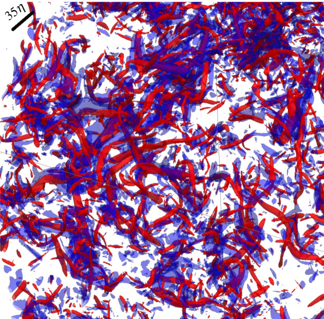
Contours of $\mathcal{Q}$ showing intense, rotational, vortex tubes (red, $\mathcal{Q}=+5\sqrt{⟨{\mathcal{Q}}^2⟩}$) enveloped by strong straining sheets (blue, $\mathcal{Q}=-2\sqrt{⟨{\mathcal{Q}}^2⟩}$), in three-dimensional homogeneous isotropic turbulence. The black scale bar at the top-left corner corresponds to a length of 35η. (Online version in colour.)

A bead–spring chain is a simple physical system that allows us to investigate the interaction between an extended filamentary object and the geometrical structure of a turbulent flow. Such a system has been widely employed in polymer physics [17] and is here generalized in order to describe a chain longer than the dissipation scale. It consists of a sequence of beads connected by phantom springs. The extensibility of the chain can be tuned by varying the strength and the maximum length of the springs, and its stiffness is controlled by a bending potential that depends on the angle between each neighbouring pair of springs. Even though a bead–spring chain can only be regarded as a very rudimentary model of an elastic filament, it has the basic properties needed to investigate the physical mechanisms that determine the motion of an extensible and flexible object in a turbulent flow. Moreover, its dynamics can be studied in detail with moderate numerical effort.

In [18], an extensible bead–spring chain was studied in a two-dimensional (2D), homogeneous, and isotropic, turbulent flow. It was shown that the centre of mass of the chain preferentially samples the vortical regions. This is because the chain is strongly stretched in high-strain regions and thus becomes unable to follow their evolution. It eventually gets trapped into one of the large-scale vortices that dominate a 2D turbulent flow. Inside the vortex, where straining is absent, it contracts and stays therein. Hence, in 2D turbulence, an extensible chain departs from straining regions but behaves like a tracer inside vortices, whence the preferential sampling of the latter.

Here we study the dynamics of a bead–spring chain in 3D turbulence, where, unlike in two dimensions, vorticity-stretching leads to the formation of intense vortex tubes [19,20], with significant straining along the tube axis. We address the question of whether preferential sampling of vortical regions persists in three dimensions and, if so, how it depends on the extensibility and flexibility of the chain.

2. Extensible chain

We consider a chain consisting of N_b identical inertialess beads (see [21] for a study of chains with inertial beads in 2D turbulent flows), each of which has a Stokes drag coefficient ζ. The beads are connected to their nearest neighbours by nonlinear springs, with equilibrium length r_eq, maximum length r_m and spring coefficient κ. The characteristic relaxation time of each spring is thus τ_E = ζ/4κ, which in turn sets the relaxation time of the chain ${\tau }_E^{\text{chain}}=(N_b+1)N_b{\tau }_E/6$ [22]. If x_i, 1 ≤ i ≤ N_b, denote the position vectors of the beads, it is convenient to describe the configuration of the chain in terms of the position of its centre of mass, ${\mathit{X}}_c=(\sum _{i=1}^{N_b}{\mathit{x}}_i)/N_b$, and the interbead separations r_j = x_j+1 − x_j, 1 ≤ j ≤ N_b − 1.

We first consider a freely jointed (the links do not oppose resistance to bending), extensible chain, as in [18]. The equations of motion for such a chain are

$${\dot{\mathit{X}}}_c=\frac{1}{N_b}\sum _{i=1}^{N_{\text{b}}}\mathit{u}({\mathit{x}}_i,t)+\frac{1}{N_b}\sqrt{\frac{r_{\text{eq}}^2}{6{\tau }_E}}\sum _{i=1}^{N_{\text{b}}}{\mathit{\xi }}_i(t)$$ 2.1a

and

$${\dot{\mathit{r}}}_j=\mathit{u}({\mathit{x}}_{j+1},t)-\mathit{u}({\mathit{x}}_j,t)+\frac{1}{\zeta }({\mathit{f}}_{j+1}^E-{\mathit{f}}_j^E)+\sqrt{\frac{r_{\text{eq}}^2}{6{\tau }_E}}\hspace{0.17em}[{\mathit{\xi }}_{j+1}(t)-{\mathit{\xi }}_j(t)],(1\le j\le N_b-1).$$ 2.1b

The elastic force on the jth bead, ${\mathit{f}}_j^E$, takes the form

$${\mathit{f}}_j^E=\kappa \hspace{0.17em}{\alpha }_j{\hat{\mathit{r}}}_j\frac{r_j}{1-r_j^2/r_m^2}-\kappa \hspace{0.17em}{\alpha }_{j-1}{\hat{\mathit{r}}}_{j-1}\frac{r_{j-1}}{1-r_{j-1}^2/r_m^2},$$ 2.2

with r_j = |r_j|, ${\hat{\mathit{r}}}_j={\mathit{r}}_j/r_j$ and

$${\alpha }_j=\{\begin{array}{ll}0& \text{if}j\le 0\hspace{0.17em}\mathrm{or}\hspace{0.17em}j=N_b\\ 1& \text{otherwise.}\end{array}$$ 2.3

The divergence of the force at r = r_m ensures that the length of the chain, $R=\sum _{j=1}^{N_b-1}{r}_j$, stays smaller than the maximum value L_m = (N_b − 1)r_m. The vectors ξ_j(t), 1 ≤ j ≤ N_b, are independent multi-dimensional white noises; they serve the purpose of modelling the collisions between the beads and the molecules of the fluid, thereby setting the equilibrium end-to-end length of the chain to $r_{\text{eq}}\sqrt{N_b-1}$. Equations (2.1) generalize the well-known Rouse model of polymer physics [17] in such a way as to account for the nonlinearity of the velocity field. Indeed, in the original Rouse model the velocity differences between the beads are replaced by their first-order Taylor expansion in the separation vectors, because polymers are assumed to be much shorter than the smallest scale of the velocity field. Here the full velocity differences are retained, since the chain is allowed to extend into the inertial range of turbulence. An analogous generalization was applied in [23–26] to the elastic dumbbell model (N_b = 2).

Finally, the velocity field u(x, t) describes the motion of the fluid and is the solution of the incompressible Navier–Stokes equations

$${\mathrm{\partial }}_t\mathit{u}+\mathit{u}\cdot \mathrm{\nabla }\mathit{u}=-\mathrm{\nabla }p+\nu \mathrm{\Delta }\mathit{u}+\mathit{F},\mathrm{\nabla }\cdot \mathit{u}=0,$$ 2.4

where p is pressure, ν the kinematic viscosity of the fluid and F(x, t) is a large-scale body forcing which maintains a homogeneous, isotropic and statistically stationary turbulent flow. We perform direct numerical simulations on a 2π-periodic domain, using a standard de-aliased pseudo-spectral method. For 3D simulations, we use a N³ = 512³ spatial grid and a second order Adams–Bashforth time-integration scheme. The body-forcing F(x, t) injects a constant amount of energy—equalling the mean dissipation rate ϵ—into the first two wavenumber shells. The Kolmogorov dissipation time and length scales are given by τ_η = (ν/ϵ)^1/2 and η = (ν³/ϵ)^1/4 ≈ 1.7 k_max (where $k_{\text{max}}=\sqrt{2}N/3$ is the maximum resolved wavenumber). The results presented below correspond to a flow with Taylor–Reynolds number $R{e}_{\lambda }=2E\sqrt{5/(3\nu ϵ)}=196$ (where E is the mean kinetic energy), which is sufficiently large for a clear inertial range (albeit less than a decade) to emerge in the energy spectrum and for the formation of distinct vortex tubes (cf. figure 1). We have checked that the sampling behaviour we describe persists even for smaller Re_λ of 123 and 64 as well, though it does intensify with Re_λ over this limited range.

While our primary focus is on chains in a 3D turbulent flow, it is helpful to compare their 3D dynamics with that in a 2D turbulent flow, especially when addressing the effects of extensibility and flexibility. For 2D flow simulations, a N² = 1024² spatial grid and a second order Runge–Kutta time-integration scheme is used, as in ref. [18]. A constant-in-time forcing F = F₀ sin(k_f x) e_y is applied, where F₀ is the forcing amplitude and k_f = 5 is the forcing wavenumber, which sets the scale of the large coherent vortices, $2\pi k_f^{-1}$. An Ekman friction term [27,28] with coefficient μ = 10⁻² is included in (2.4) to damp out the energy at the large scales (due to an inverse cascade).

After the flow (3D or 2D) attains a stationary state, we introduce a large number of chains, of order 10⁴, each with N_b = 20 beads. We evolve many chains simultaneously only to obtain good statistics; the dynamics we study are of a single chain in the flow. The chains are given a small initial length, close to the no-flow equilibrium value. They are then allowed to be stretched out by the flow and attain a steady-state distribution before we begin recording statistics. The equations governing the dynamics of the centre of mass and separation vectors of the chain are integrated using a second-order Runge–Kutta scheme, augmented by a rejection algorithm [29] that prevents the nonlinear spring force from diverging as |r| approaches r_m. The chains are evolved with a time step Δt_chain = Δt_f/N_sub, where Δt_f is the time-step of the fluid flow solver and N_sub is the number of sub-steps taken by the chain solver for every step of the fluid solver. The flow is assumed to be unchanging over the duration of the sub-steps. While N_sub is set to unity for the freely-jointed chain, used in this section, we use up to N_sub = 10³ for accurately resolving the numerically-stiff dynamics of inextensible and inflexible chains, to be introduced later in §§3 and 4.

The influence of elasticity on the dynamics of the chain is described in terms of the elastic Weissenberg number ${\mathit{\text{Wi}}}_E={\tau }_E^{\text{chain}}/{\tau }_f$, which is the ratio of the chain relaxation time to the viscous-dissipation time scale of the flow. For 3D turbulence, ${\tau }_f={\tau }_{\eta }$, whereas for 2D flows we choose the small time scale associated with the dissipation of enstrophy, τ_f = 〈2ω²〉^−1/2, where 〈ω²〉 is the mean enstrophy. For small Wi_E, the chain is in a contracted configuration and acts like a tracer; for large Wi_E, it is stretched out by the flow.

As mentioned in §1, the dynamics of an extensible chain was studied in [18] for a 2D turbulent flow forced at large spatial scales. The equilibrium size of the chain was assumed to be of the order of the dissipation scale, while L_m was much longer and comparable to the scale of the coherent vortices, $2\pi k_f^{-1}$, or even greater than it. When Wi_E was sufficiently large for the typical length of the chain to approach the size of the vortices, then the chain was shown to exhibit a marked preferential sampling of vortical regions. The mechanism that was proposed in [18] to explain this phenomenon, already sketched briefly in §1, can be summarized as follows:

• Inside a vortex, where stretching is absent, the chain shrinks down to its equilibrium size. Since the equilibrium size of the chain is much smaller than the size of the vortex, the chain essentially behaves as a tracer and follows the vortex during its lifetime.

• In a region of intense strain, the chain is stretched to the extent that it cannot continue to follow the straining region. The chain eventually encounters a vortex that coils it up and ‘entraps’ it according to the dynamics described above.

The combination of these effects causes an extensible chain to stay inside large vortices and leave high-strain regions, which results in a strong preferential sampling of vortices. This phenomenon was quantified in [18] by studying the Okubo–Weiss parameter [30,31] evaluated at the position of the centre of mass of the chain,

$${\mathrm{\Lambda }}_c=\frac{{\omega }_c^2-{\sigma }_c^2}{4⟨{\omega }^2⟩},$$ 2.5

where ω_c and σ_c are the vorticity and the strain rate at the position of the centre of mass, respectively. We recall that positive values of Λ_c correspond to vorticity-dominated regions, whereas negative values indicate strain-dominated regions. For large enough values of Wi_E, the probability of positive values of Λ_c was found to be much higher than for a tracer transported by the same flow [18]. In addition, the joint probability density function (PDF) of the chain length R and Λ_c confirmed that the chain is contracted in vortical regions and extended in straining ones.

The first question we address here is whether or not an extensible chain exhibits preferential sampling of vortical regions also in a 3D turbulent flow. A substantial difference indeed exists between 2D and 3D flows. A 2D turbulent flow is characterized by large, long-lived vortices, inside which stretching is weak. In a 3D turbulent flow, vorticity concentrates into intense tubular structures with significant stretching along their axes. The dynamics of the chain in vorticity-dominated regions is therefore expected to be substantially different in the two cases.

In three dimensions, the local nature of the flow can be classified by using the $\mathcal{Q}$-$\mathcal{R}$ representation of the velocity gradient [32]. If $A_c={\tau }_{\eta }\mathrm{\nabla }\mathit{u}({\mathit{X}}_c(t),t)$ denotes the rescaled velocity gradient at the position of the centre of mass, let ${\mathcal{Q}}_c=-\mathrm{tr}{\mathsf{A}}_c^2/2$ and ${\mathcal{R}}_c=-\det {\mathsf{A}}_c$ be its second and third invariants. Since ${\mathcal{Q}}_c$ can be rewritten as

$${\mathcal{Q}}_c={\tau }_{\eta }^2\frac{{\omega }_c^2/2-{\mathsf{S}}_c:{\mathsf{S}}_c}{2};{\mathsf{S}}_c=\frac{({\mathsf{A}}_c+{\mathsf{A}}_c^{\text{T}})}{2},$$ 2.6

the sign of ${\mathcal{Q}}_c$ discriminates between the regions dominated by vorticity (${\mathcal{Q}}_c>0$) and those dominated by strain (${\mathcal{Q}}_c<0$). Thus, ${\mathcal{Q}}_c$ has a role analogous to that played by Λ_c in a 2D flow. Figure 1 presents a snapshot of the iso-surfaces of $\mathcal{Q}$ from our 3D simulation, which clearly reveal sheet-like straining zones (large negative $\mathcal{Q}$ in blue) in close proximity to intense tubular vortices (large positive $\mathcal{Q}$ in red).

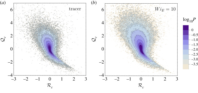
Figure 2 compares the steady-state joint PDFs of ${\mathcal{R}}_c$ and ${\mathcal{Q}}_c$ for a tracer particle (panel a) and for the extensible chain with a large Wi_E = 10 (figure 2b). The chain has an equilibrium size of about 0.4η and a maximum extension L_m = 40η, so that when the chain is stretched its length R lies in the inertial range and is comparable to the typical size of vortex tubes in our simulations (cf. the vortex tubes and scale bar in figure 1). The shape of the joint PDF of the chain is similar to that of the tracer. However, the probability of sampling positive ${\mathcal{Q}}_c$ is significantly larger for the chain, than for the tracer. Therefore, we deduce that preferential sampling of vorticity-dominated regions persists in three dimensions.

Figure 2.

Joint PDF of ${\mathcal{R}}_c$ and ${\mathcal{Q}}_c$ (a) for a tracer and (b) for an inertialess, freely jointed, extensible chain with Wi_E = 10, L_m = 40η, r_eq = 0.045η. (Online version in colour.)

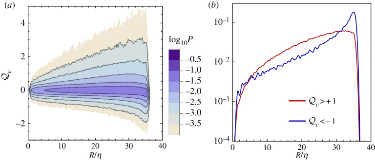
As mentioned above, however, a major difference exists between the chain dynamics in 2D and 3D turbulence. This is reflected in the conditional PDF of the chain length R given the value of ${\mathcal{Q}}_c$, presented in figure 3b, which shows that contrary to the 2D case the chain is considerably stretched not only in strain-dominated but also in vorticity-dominated regions. This difference is clear from the comparison of the joint PDF of R and ${\mathcal{Q}}_c$, shown in figure 3a, with its 2D analogue (see fig. 3 in [18]) and has important consequences for preferential sampling. In two dimensions, indeed, the contraction of the chain inside vortices was identified as an essential element of the sampling dynamics [18] (though we shall revisit this idea in §4). In three dimensions, the chain does not collapse into a tracer even when the flow has a strong vortical nature (figure 3b). Hence, the mechanism leading to preferential sampling ought to be different from that operating in 2D turbulence.

Figure 3.

(a) Joint PDF of the chain length R (rescaled by the dissipation scale η) and ${\mathcal{Q}}_c$ for a freely jointed inextensible chain. (b) Conditional PDF of R rescaled by η given ${\mathcal{Q}}_c<-1$ (blue curve) and ${\mathcal{Q}}_c>1$ (red curve). The parameters are Wi_E = 10, L_m = 40η, r_eq = 0.045η in both panels. (Online version in colour.)

Now, the only way an elongated chain can remain inside a vortex tube of comparable length, is if it aligns itself along the vortex axis. Given that the majority of vortices are axially stretched (figure 2), this scenario is consistent with our observation that the chain is typically stretched out inside a vortex (figure 3b). In contrast, it is unlikely that the entire chain can be encapsulated into straining regions, given their less coherent, sheet-like topology. Moreover, the evolution of straining regions is much more non-local in nature than that of the vortex tubes [33], which tend to move with the fluid, except for the effects of viscous diffusion (in the inviscid limit the tubes would be ‘frozen’ into the fluid as a consequence of Kelvin’s circulation theorem [20]). Thus, we expect a chain to be able to enter and follow a vortex tube more easily than a straining region.

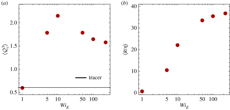
This explanation implies that there is an ideal chain elasticity for preferential sampling: if Wi_E is too small then the chain acts like a tracer, whereas, if Wi_E is too large then the chain may stretch out beyond the length of the vortex tubes and be unable to reside inside them. This intuition is corroborated by figure 4, which shows the effect of Wi_E on preferential sampling (figure 4a), as well as on the mean length of the chain (figure 4b). We find that the third moment of the PDF of ${\mathcal{Q}}_c$, whose positivity implies a higher probability of positive ${\mathcal{Q}}_c$, varies non-monotonically with Wi_E, peaking at a value which corresponds to a mean chain length 〈R〉 ≈ 20η. For larger Wi_E, all the chains approach the maximum chain length L_m = 40η and cannot reside within the vortex tubes as effectively (cf. figure 1).

Figure 4.

(a) Third moment of the distribution of ${\mathcal{Q}}_c$ and (b) the average chain length as a function of Wi_E, for fixed L_m = 40η and r_eq = 0.045η. The value of $⟨{\mathcal{Q}}_c^3⟩$ for a tracer is shown as a horizontal black line in a; it is positive due to the presence of intense vortex tubes. (Online version in colour.)

We shall present more direct evidence for our explanation of 3D preferential sampling in §4. But first, let us address the question that naturally arises from figure 3a: Is elasticity essential for preferential sampling, given that the chains are stretched out even inside vortices? The physical picture of chains aligning along vortex tubes would hold even for long chains of a fixed length, and so we would expect such inextensible chains to show preferential sampling as well. We test this idea in the next section.

3. Inextensible chain

In order to describe a ‘macroscopic’ inextensible chain, we disregard Brownian fluctuations in (2.1) and replace ${\mathit{f}}_j^E$ with

$${\tilde{\mathit{f}}}_j^E=\kappa \hspace{0.17em}{\alpha }_j{\hat{\mathit{r}}}_j(r_j-r_{\text{eq}})-\kappa \hspace{0.17em}{\alpha }_{j-1}{\hat{\mathit{r}}}_{j-1}(r_{j-1}-r_{\text{eq}}),$$ 3.1

where r_eq still has the meaning of equilibrium length of the springs. Wi_E is set to a very small value to ensure that the chain is in effect inextensible. Its length is then L = (N_b − 1)r_eq (in the simulations, we set Wi_E = 0.1, which ensures that $R=\sum _{j=1}^{N_b-1}{r}_j$ differs from L by 2% at most).

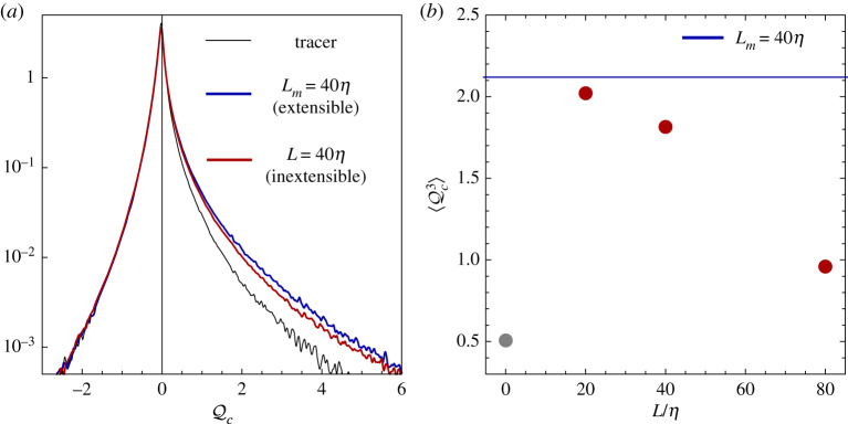
We now consider an inextensible chain having the same length as the maximum length of the extensible chain (with Wi_E = 10) considered in §2, i.e. we take L = L_m = 40η. The PDFs of ${\mathcal{Q}}_c$ for the two cases are compared in figure 5a. The absence of extensibility is seen to have only a small effect.

Figure 5.

(a) PDF of ${\mathcal{Q}}_c$ for a tracer (black curve), an extensible chain with Wi_E = 10, r_eq = 0.045η and L_m = 40η (blue curve), and an inextensible chain with L = L_m (red curve). (b) Third moment of the PDF of ${\mathcal{Q}}_c$ for a tracer (grey bullet) and for an inextensible chain with various lengths L (red bullets). The blue line indicates the value of $⟨{\mathcal{Q}}_c^3⟩$ for the extensible chain of a. The mean length of this extensible chain is close to 20η, as seen in figure 4b (case of Wi_E = 10). (Online version in colour.)

The influence of the length L of the inextensible chain on the level of preferential sampling is depicted in figure 5b, in terms of the third moment of ${\mathcal{Q}}_c$. Here, we see the same non-monotonic variation of $⟨{\mathcal{Q}}_c^3⟩$ with L, that we saw with Wi_E for the extensible chain (figure 4a). Moreover, the value of $⟨{\mathcal{Q}}_c^3⟩$ for L = 20η is very close to that of the extensible chain (horizontal line in panel b), which has a mean length 〈R〉 ≈ 20η (case of Wi_E = 10 in figure 4b). These results clearly demonstrate that preferential sampling persists even when the chain is not collapsible. Indeed the only role of extensibility is to allow a chain with a short equilibrium length to be stretched by the flow and reach the appropriate length for staying in a vortex; it does not influence the preferential-sampling dynamics otherwise. This finding supports our intuition regarding the mechanism of preferential sampling whereby the chain resides in intense vortical regions by aligning with the axis of vortex tubes. Such a mechanism, indeed, does not rely on the extensibility of the chain, and is equally applicable to inextensible, but long, chains.

The results in figure 5b also confirm our understanding of figure 4b, that there is an optimal length for preferential sampling—either attained dynamically by stretching or permanently fixed from the outset—that is comparable to the characteristic linear size of vortex tubes.

4. Inflexible chain

So far we have considered a chain that does not oppose bending. However, taking the bending stiffness of the chain into account allows us to further understand preferential sampling in 3D turbulence. Specifically, by increasing the stiffness of the chain, we can check whether it is necessary for chains to be able to coil in order to enter vortex tubes. Coiling certainly plays an important role in preferential sampling in 2D turbulence, as demonstrated indirectly in [18], where the deformability of the chain was controlled by changing the number of beads N_b while keeping the maximum length L_m fixed. Here, we directly incorporate the forces arising from bending stiffness into the equations of motion, by assuming that the chain has a bending energy given by [34]

$$E^B=A{r}_{\text{eq}}^{-1}\sum _{j=2}^{N_b-1}(1-{\hat{\mathit{r}}}_j\cdot {\hat{\mathit{r}}}_{j-1}),$$ 4.1

where A > 0 determines the bending stiffness.¹ The bending energy generates a force that depends on the angle between two neighbouring links and whose effect is to restore the chain into a rod-like configuration. The form of the force on the jth bead is [34]

$$\begin{array}{rl}{\mathit{f}}_j^B& =\frac{A}{r_{eq}}[\frac{{\alpha }_{j-2}}{r_{j-1}}\hspace{0.17em}{\hat{\mathit{r}}}_{j-2}-(\frac{{\alpha }_{j-2}}{r_{j-1}}\hspace{0.17em}{\hat{\mathit{r}}}_{j-2}\cdot {\hat{\mathit{r}}}_{j-1}+\frac{{\alpha }_{j-1}}{r_j}+\frac{{\alpha }_{j-1}}{r_{j-1}}\hspace{0.17em}{\hat{\mathit{r}}}_{j-1}\cdot {\hat{\mathit{r}}}_j){\hat{\mathit{r}}}_{j-1}\\ \hspace{0.17em}& +(\frac{{\alpha }_{j-1}}{r_j}\hspace{0.17em}{\hat{\mathit{r}}}_{j-1}\cdot {\hat{\mathit{r}}}_j+\frac{{\alpha }_{j-1}}{r_{j-1}}+\frac{{\alpha }_j}{r_j}\hspace{0.17em}{\hat{\mathit{r}}}_j\cdot {\hat{\mathit{r}}}_{j+1}){\hat{\mathit{r}}}_j-\frac{{\alpha }_j}{r_j}{\hat{\mathit{r}}}_{j+1}],\end{array}$$ 4.2

where α_j was defined in (2.3). The characteristic time associated with this force is ${\tau }_B=\zeta r_{\text{eq}}^3/A$, and a dimensionless measure of it is the ‘bending’ Weissenberg number ${\mathit{\text{Wi}}}_B={\tau }_B/{\tau }_{\eta }$. The chain is inflexible and rod-like for small Wi_B, while the freely-jointed limit is recovered for large Wi_B.

With the addition of the bending stiffness, the evolution equations for an inertialess, inextensible chain become

$${\dot{\mathit{X}}}_c=\frac{1}{N_b}\sum _{i=1}^{N_{\text{b}}}\mathit{u}({\mathit{x}}_i,t)$$ 4.3a

and

$${\dot{\mathit{r}}}_j=\mathit{u}({\mathit{x}}_{j+1},t)-\mathit{u}({\mathit{x}}_j,t)+\frac{1}{\zeta }({\tilde{\mathit{f}}}_{j+1}^E-{\tilde{\mathit{f}}}_j^E)+\frac{1}{\zeta }({\mathit{f}}_{j+1}^B-{\mathit{f}}_j^B)(1\le j\le N_b-1).$$ 4.3b

We begin by assessing the effect of bending stiffness on preferential sampling in two dimensions. As we already appreciate the importance of coiling in two dimensions [18], studying the impact of bending stiffness in this case will help us better understand the results in three dimensions. Moreover, this also provides us with the opportunity to check whether extensibility is crucial for preferential sampling in two dimensions as suggested in [18], i.e., whether it is essential for a chain inside a vortex to collapse to a tracer, or if it is sufficient for a long chain to simply coil into the vortex.

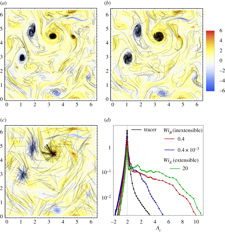
Figure 6 presents snapshots of the inextensible chains overlaid on the vorticity field, for a highly flexible (figure 6a), a moderately flexible (figure 6b), and an inflexible (figure 6c) case (online movie of highly flexible chains in 2D turbulence: https://youtu.be/22X0Gt5y2cM; online movie of moderately flexible chains: https://youtu.be/j-c8eLjeECM; Online movie of inflexible chains: https://youtu.be/HanNeqaqya8. They are also available as electronic supplementary material). We see that the highly flexible chain is coiled up by the vortices and stays almost entirely within them. The inflexible rod-like chain, however, is unable to coil, and thus while some portions of the chain linger within vortices, the entire chain can never be entrapped by a vortex and preferential sampling weakens considerably. This effect of bending stiffness, which is exactly as anticipated in [18], is shown quantitatively by the PDFs of Λ_c in figure 6d (see (2.5) for the definition of Λ_c). An analogous behaviour is observed for inextensible, inertialess fibres, described by the local slender-body theory, in a two-dimensional turbulent flow (Jérémie Bec, 2018 personal communication).

Figure 6.

Snapshots of an ensemble of inextensible chains (black lines) in a 2D turbulent flow, overlaid on the vorticity field, corresponding to (a) Wi_B = 0.4 (highly flexible), (b) Wi_B = 0.4 × 10⁻¹ (moderately flexible) and (c) Wi_B = 0.4 × 10⁻³ (inflexible). It should be noted that several chains are plotted at the same time in order for the reader to visualize the preferential sampling of vortices more easily. There is, however, no interaction between the chains. The length of the chain L is equal to the large vortex scale 2π/k_f = 1.25. (d) PDF of the Okubo–Weiss parameter for the inextensible chain of panels a and c, along with the PDF for a tracer, as well as that for an extensible chain (Wi_E = 20) with equilibrium size of 0.04 and maximum length L_m equal to the length L of the inextensible chain. (Online version in colour.)

Figure 6d also allows us to address the role of extensibility in two dimensions, by comparing the PDF of Λ_c for an extensible, freely jointed, chain (Wi_E = 20, studied in [18]) with the PDF for the inextensible, highly flexible chain (Wi_B = 0.4). The extensible chain has a small equilibrium length of 0.04 and a maximum length L_m = 1.25, which equals the fixed length L of the inextensible chain. We see that while there is a small reduction of the degree of preferential sampling when the chain is unable to collapse to a tracer-like object, the long inextensible chains are still able to occupy vortices effectively (figure 6a), provided of course that they are flexible. Therefore, extensibility is not a crucial ingredient for preferential sampling, either in two dimensions or in three dimensions (shown in §3). However, it does have a more significant effect in two dimensions because extensible chains can collapse to tracers inside 2D vortices, whereas this is not possible inside axially stretched 3D vortex tubes.

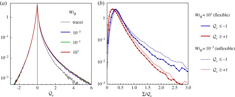
Returning to the effect of the bending stiffness, we have shown above that in two dimensions it strongly affects the preferential sampling of vortical regions because chains must coil in order to enter vortices. We now examine the effect of the bending stiffness in three dimensions. Figure 7a shows the PDF of ${\mathcal{Q}}_c$ for a long inextensible chain (L = 20η) with different values of Wi_B, corresponding to a highly flexible (Wi_B = 10¹), a moderately flexible (Wi_B = 10⁻¹) and a rod-like inflexible (Wi_B = 10⁻³) chain. The PDF clearly does not vary with Wi_B, which is an unequivocal indication that, in three dimensions, the bending stiffness has no effect on preferential sampling. This fact provides further confirmation of our explanation of preferential sampling of vortical regions in 3D turbulence. If the main mechanism is the alignment of the chain with the axis of the tubular structures on which vorticity concentrates, the chain does not need to coil in order to reach and keep that configuration. It is then natural that the bending stiffness does not affect preferential sampling in three dimensions.

Figure 7.

(a) PDF of ${\mathcal{Q}}_c$ for a tracer and for an inextensible chain (L = 20η) with bending stiffness varying from that of a highly flexible chain (Wi_B = 10¹) to that of a rod-like inflexible one (Wi_B = 10⁻³). (b) PDF of the standard deviation Σ of the values of ${\mathcal{Q}}_j$ sampled by the beads of a chain, conditioned on the centre of mass being in a vortical (${\mathcal{Q}}_c\ge +1$) or straining region (${\mathcal{Q}}_c\le -1$). Results are shown for the cases of a highly flexible (Wi_B = 10¹) and inflexible (Wi_B = 10⁻³) chain of panel a. (Online version in colour.)

All our results, thus far, point to the ability of chains to thread vortex tubes and follow them by aligning with the vortex axis. In contrast, no such mechanism exists for chains to reside inside straining zones which have a complex geometry and evolve non-locally, as pointed out earlier in §2. Indeed this difference between vortical and straining regions forms the basis for our explanation of preferential sampling. Therefore, it is important to support this claim with some direct evidence. To this end, we denote by ${\mathcal{Q}}_j$ the value of $\mathcal{Q}$ at the position of the jth bead, x_j. We then consider the mean μ and standard deviation Σ of ${\mathcal{Q}}_j$ over the N_b beads of the chain

$$\mu ={⟨{\mathcal{Q}}_j⟩}_b\text{and}\mathrm{\Sigma }=⟨{({\mathcal{Q}}_j-\mu )}^2{⟩}_b^{1/2}$$ 4.4

with 〈 · 〉_b denoting the average over j = 1, …, N_b. Figure 7b compares the conditional PDFs of Σ for chains in rotational (${\mathcal{Q}}_c\ge +1$) and straining (${\mathcal{Q}}_c\le -1$) regions, for both flexible and inflexible (inextensible) chains. In both cases, we see that Σ is typically greater when the centre of mass of the chain is in a high-strain region. This finding confirms that it is generally easier for a chain, even if it is rod-like, to reside within vortex tubes than within straining regions.

5. Concluding remarks

We have shown that a long bead–spring chain—a simple model for filamentary objects—preferentially samples vortical regions of both two dimensions and three dimensions turbulent flows. This behaviour is exhibited by a long inextensible chain, as well as an extensible one that has a small equilibrium length but which is stretched out to inertial-range scales by the flow. The key difference between the underlying mechanisms in two dimensions and three dimensions is revealed by the contrasting behaviour of inflexible chains. In two dimensions, where the chain must coil in order to be trapped within vortices, bending stiffness inhibits preferential sampling. In three dimensions, however, an inflexible chain exhibits the same sampling behaviour as a fully flexible one, because the chain follows tubular vortices by aligning with their axes, and neither bending nor extensibility is essential for this to occur.

The extent of preferential sampling is much stronger in 2D than in 3D turbulence (compare the difference between the PDFs for a tracer and the chain in figure 6d and figure 7a). This is because 2D coherent vortices have much longer lifetimes than 3D vortex tubes, allowing the chain to spend a much larger fraction of time inside the former. On the other hand, the preferential sampling phenomenon is more robust in 3D, as it persists regardless of the extensibility or flexibility of the chain.

Filamentary objects in turbulent flows are encountered in several physical situations, from fibres in the paper industry to micro-plastics and algae in oceanic environments. The understanding of the sampling behaviour of individual chains developed here sets the stage for future studies of the transport, dispersion and settling of filaments in turbulent suspensions, for which, however, additional physical effects such as intra-chain and inter-chain hydrodynamic interactions must be considered.

Data accessibility

The data shown in this paper (and a sample analysis code along with a ReadMe explanatory file about how to process the data on any platform) is available on figshare at https://figshare.com/articles/Elastic_Chains_Data_and_code/11955612.

Authors' contributions

J.R.P., S.S.R. and D.V. conceived of the problem; the simulations were carried out by J.R.P. and the analysis by D.V., R.S. and J.R.P. The draft was written by D.V. and J.R.P. All authors read and approved the manuscript.

Competing interests

The authors declare that they have no competing interests.

Funding

J.R.P., S.S.R. and D.V. acknowledge the support of the Indo-French Centre for Applied Mathematics (IFCAM). J.R.P. acknowledges funding from the IITB-IRCC seed grant. S.S.R. and R.S. acknowledge support of the DAE, Govt. of India, under project no. 12-R&D-TFR-5.10-1100. S.S.R. also acknowledges DST (India) project MTR/2019/001553 for support.