. 2020 Jun 26;9:e53445. doi: 10.7554/eLife.53445

Figure 2. Calculating the stimulus-dependent dynamic spectrotemporal receptive field.

(A) Activation of nodes in a neural network with rectified linear (ReLU) nonlinearity for the stimulus at time t. (B) Calculating the stimulus-dependent dynamic spectrotemporal receptive field (DSTRF) for input instance Xt by first removing all inactive nodes from the network and replacing the active nodes with the identity function. The DSTRF is then computed by multiplying the remaining network weights. Reshaping the resulting weight matrix expresses the DSTRF in the same dimensions as the input stimulus and can be interpreted as a multiplicative template applied to the input. Contours indicate 95% significance (jackknife). (C) Comparison of piecewise linear (rectified linear neural network) and linear (STRF) approximations of a nonlinear function. (D) DSTRF vectors (columns) shown for 40 samples of the stimulus. Only a limited number of lags and frequencies are shown at each time step to assist visualization. (E) Normalized sorted singular values of the DSTRF matrix show higher diversity of the learned linear function in STG sites than in HG sites. The bold lines are the averages of sites in the STG and in HG. The complexity of a network is defined as the sum of the sorted normalized singular values. (F) Comparison of network complexity and the improved prediction accuracy over the linear model in STG and HG areas. (G) Histogram of the average number of switches from on/off to off/on states at each time step for the neural sites in the STG and HG.

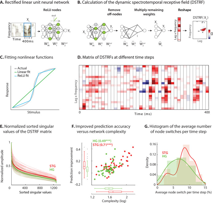
Figure 2—source data 1. A MATLAB file containing one variable — complexity (neural network complexity, as used in Figure 5A prediction).

Figure 2.

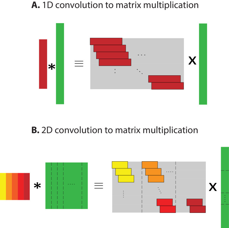
Figure 2—figure supplement 1. Converting convolution to matrix multiplication.

Figure 2—figure supplement 1.

Converting the convolutional neural networks into a feedforward network helps simplify DSTRF calculation. The convolution operation is linear; hence, it can be converted into a matrix multiplication. (A) Converting 1-d convolution into a 2-d matrix multiplication. The matrices are the shifted version of the 1-d vectors. The i-th row in the output will be the product of the input vectors (shown in green) and the convolution kernel (red) shifted by i steps. (B) Converting 2-d convolution to a 2-d weight matrix using the same principle by flattening both the kernel and the input into one-dimensional forms by stacking the columns vertically on top of each other.
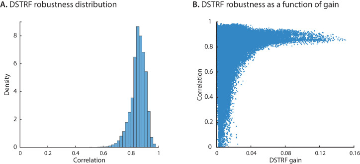
Figure 2—figure supplement 2. DSTRF robustness across initializations.

Figure 2—figure supplement 2.

We trained 10 instances of the CNN model for each electrode and grouped them into two groups of evens and odds. For all time points, we calculated the 2D correlation of the average DSTRF from the even models with the average DSTRF from the odd models. (A) A histogram of all values where one data point corresponds to the robustness for a specific electrode at a specific time point. (B) The relation of robustness with the gain of the linearized function. When the DSTRF has higher gain the function is more robust.
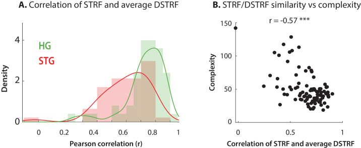
Figure 2—figure supplement 3. Comparing DSTRFs to STRFs.

Figure 2—figure supplement 3.

(A) The average DSTRF calculated across the test dataset is highly correlated with the calculated STRF, especially for HG electrodes. (B) Similarity of STRF and the average DSTRF is inversely correlated with the complexity of the function the CNN model has learned, as expected. Each data point is an electrode and the R-value represents Spearman correlation.